Affiliation Networks

Two-Mode Networks, Bipartite Graphs, and the Duality of Persons and Groups

Part 1: What Are Affiliation Networks?

Networks of a Different Kind

  • Typically, a network consists of a set of units of the same kind linked via some kind of relationship:
    • Person to person friendship ties
    • Organization to organization alliances
    • Airport to airport plane routes
  • But sometimes a network is composed of relationships between two types of entities:
    • Persons and the groups they belong to
    • Actors and the movies they appear in
    • Scientists and the papers they write
  • These are called Affiliation Networks

What Gets Studied as an Affiliation Network?

Types of affiliation networks that have been studied in the literature include:

  • Hollywood actors and the movies that they make
  • CEOs and the boards of directors that they sit on
  • Books and the people who buy them
  • Scientists and the journals/papers they publish in
  • Students and the clubs they join
  • The corporate interlock network is a classic example (Mizruchi 1983):
    • When the same executive sits on multiple company boards, companies end up connected through shared people
    • Most big corporations end up forming part of a single giant network

A Real Affiliation Network: Corporate Interlocks

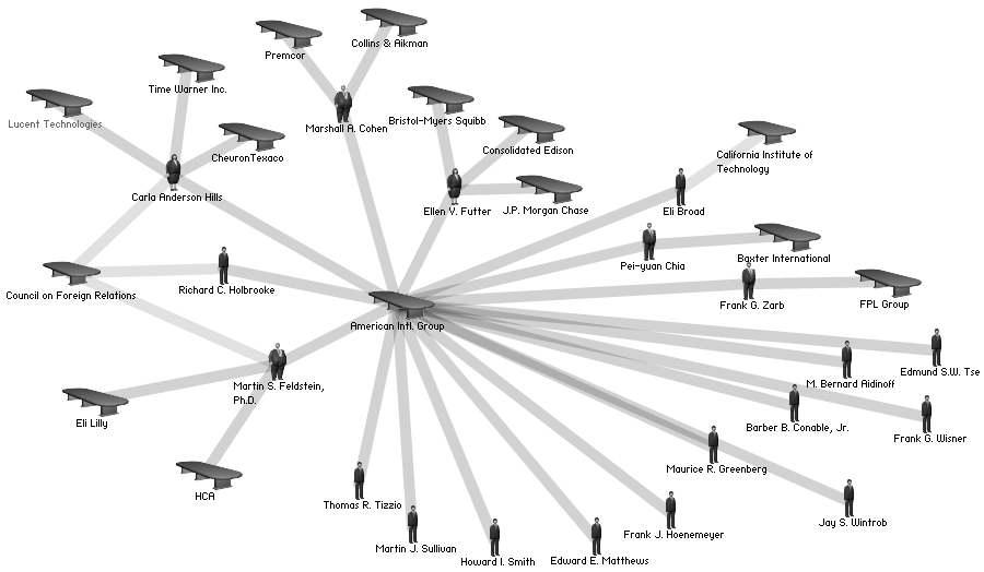
  • AIG’s board, 2004: each director (person icon) shown with the other corporations they serve (boardroom tables)
  • Exactly the bipartite structure from the previous slides: two node sets — directors and boards
  • Shared directors connect companies: Ellen Futter’s seats link J.P. Morgan Chase, Bristol-Myers Squibb, and Consolidated Edison
  • This is the corporate interlock network: companies tied through the people they share

Image: TheyRule.net via Wikimedia Commons (CC0)
Part 1: From Theory to Graph to Matrix

The Three-Step Shuffle

How a sociological idea becomes a network measure:

1. Theory

Begin with theories specifying the membership relation between people and other entities: groups, teams, events.

→

2. Graph

Translate the membership concept into a graph-theoretic concept: the bipartite graph.

→

3. Matrix

Link the bipartite graph to matrix algebra to come up with network-analytic measures (e.g., centralities of individuals and events).

Affiliation Networks and Two-Mode Networks

  • The general relationship between people and the larger entities they join is called an affiliation
  • Networks linking people to the groups, projects, and events they join are affiliation networks
  • Affiliation networks are a special case of the larger class of two-mode networks: networks with two types of vertices
  • Two-mode networks are, in turn, a subset of multi-mode networks: networks with more than two types of vertices
  • Note that the plain old graphs featuring only one type of node we have been dealing with all along are technically called unipartite graphs

Part 2: Bipartite Graphs

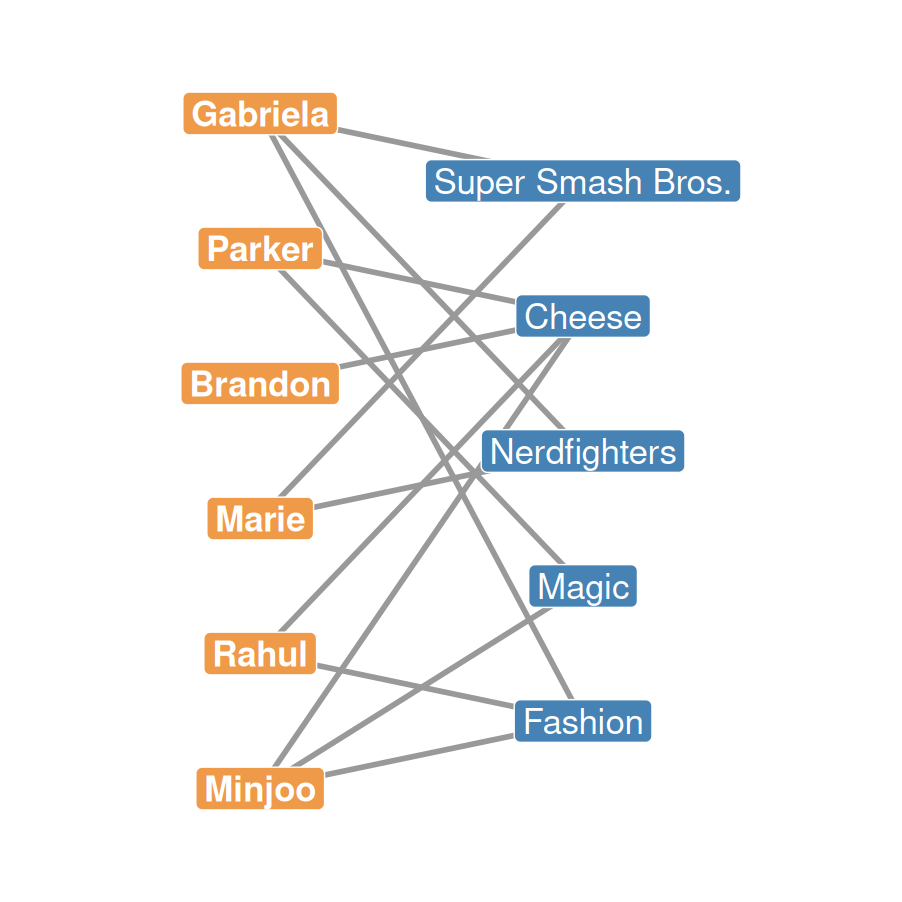
The Running Example: Students and Clubs

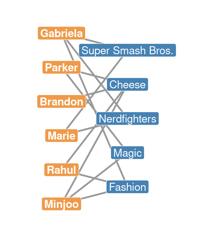
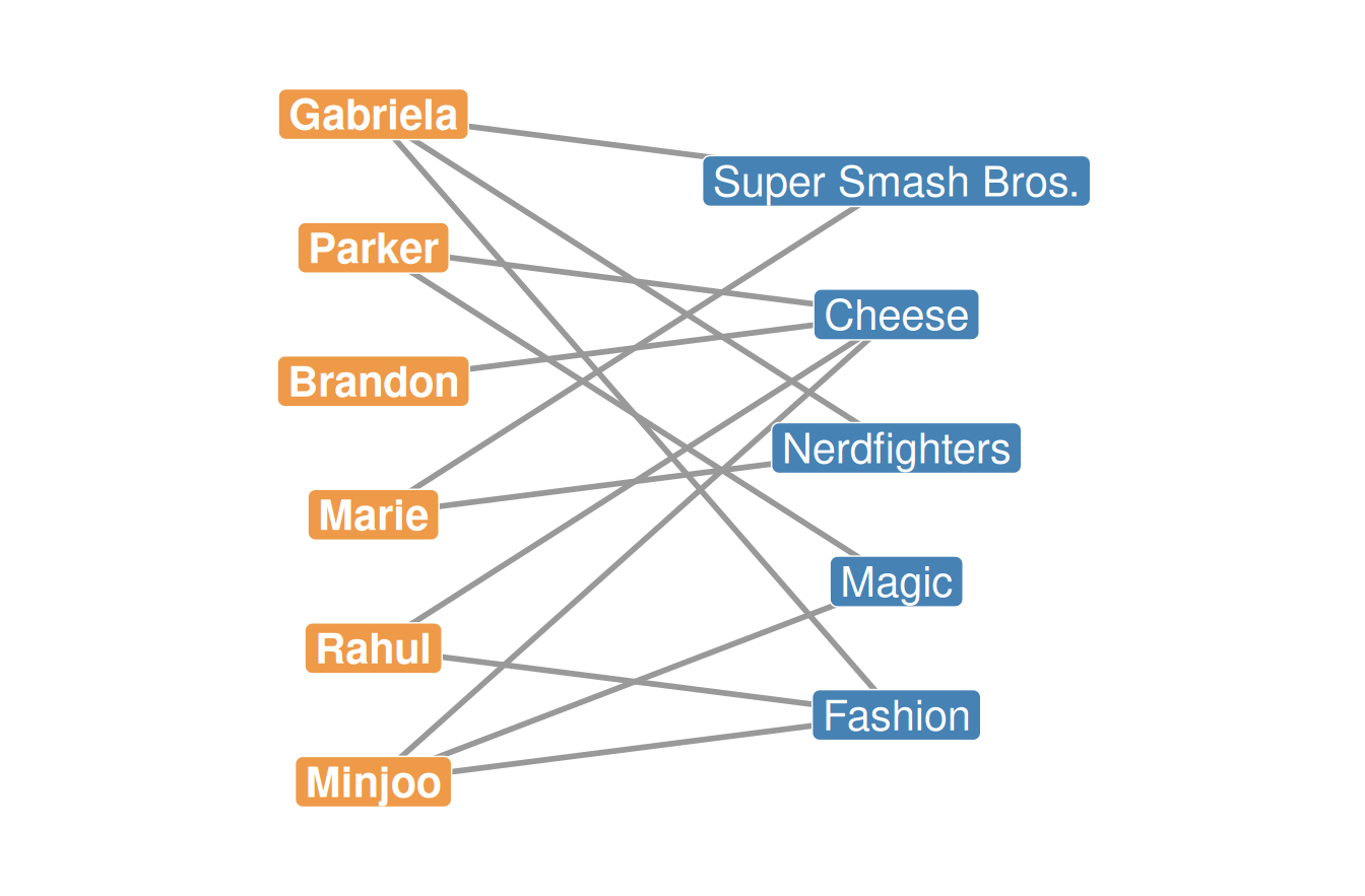
  • Six students and the five college activity clubs they belong to

Bipartite Graphs

  • A bipartite graph is a special kind of graph featuring:
    • Two disjoint sets of vertices, \(U\) and \(V\)
      • Two sets are disjoint when they don’t share members
    • One edge set (\(E\)): \(G_B = \{E, U, V\}\)
    • Edges link vertices between sets but not within sets
    • The two vertex sets can be of different cardinality!
      • \(|U| = 6\) people, \(|V| = 5\) clubs in our example
  • Affiliation or membership relations are undirected
    • If person \(i\) is a member of club \(j\), then club \(j\) has person \(i\) as a member — the relation is symmetric by definition
Node Neighborhoods in Bipartite Graphs

  • Node neighborhoods work like in regular graphs, except:
    • The neighbors of nodes from set \(U\) are always members of set \(V\) (and vice versa)

\[N(\text{Minjoo}) = \{\text{Cheese, Magic, Fashion}\}\] \[N(\text{Gabriela}) = \{\text{Super Smash Bros., Nerdfighters, Fashion}\}\]

  • The intersection of their neighborhoods:
    • \(N(\text{Minjoo}) \cap N(\text{Gabriela}) = \{\text{Fashion}\}\) — one shared club, a first hint of the overlap idea to come!
  • The union of their neighborhoods:
    • \(N(\text{Minjoo}) \cup N(\text{Gabriela})\) = {Super Smash Bros., Cheese, Nerdfighters, Magic, Fashion} — all five clubs touched between them!
Neighborhoods of the Other Mode

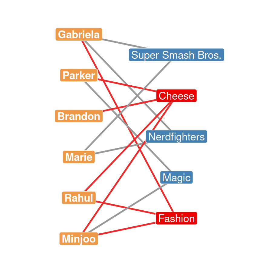
  • Both sets of nodes have neighborhoods!

\[N(\text{Cheese}) = \{\text{Parker, Brandon, Rahul, Minjoo}\}\] \[N(\text{Fashion}) = \{\text{Gabriela, Rahul, Minjoo}\}\]

  • The intersection:
    • \(N(\text{Cheese}) \cap N(\text{Fashion}) = \{\text{Rahul, Minjoo}\}\)
    • The two clubs share two members
  • The union: \(N(\text{Cheese}) \cup N(\text{Fashion})\) = {Gabriela, Parker, Brandon, Rahul, Minjoo} — five of the six students, everyone but Marie
  • Same-kind nodes cannot be connected in a two-mode network (by construction) — but they can share neighbors
Node Degree in Bipartite Graphs
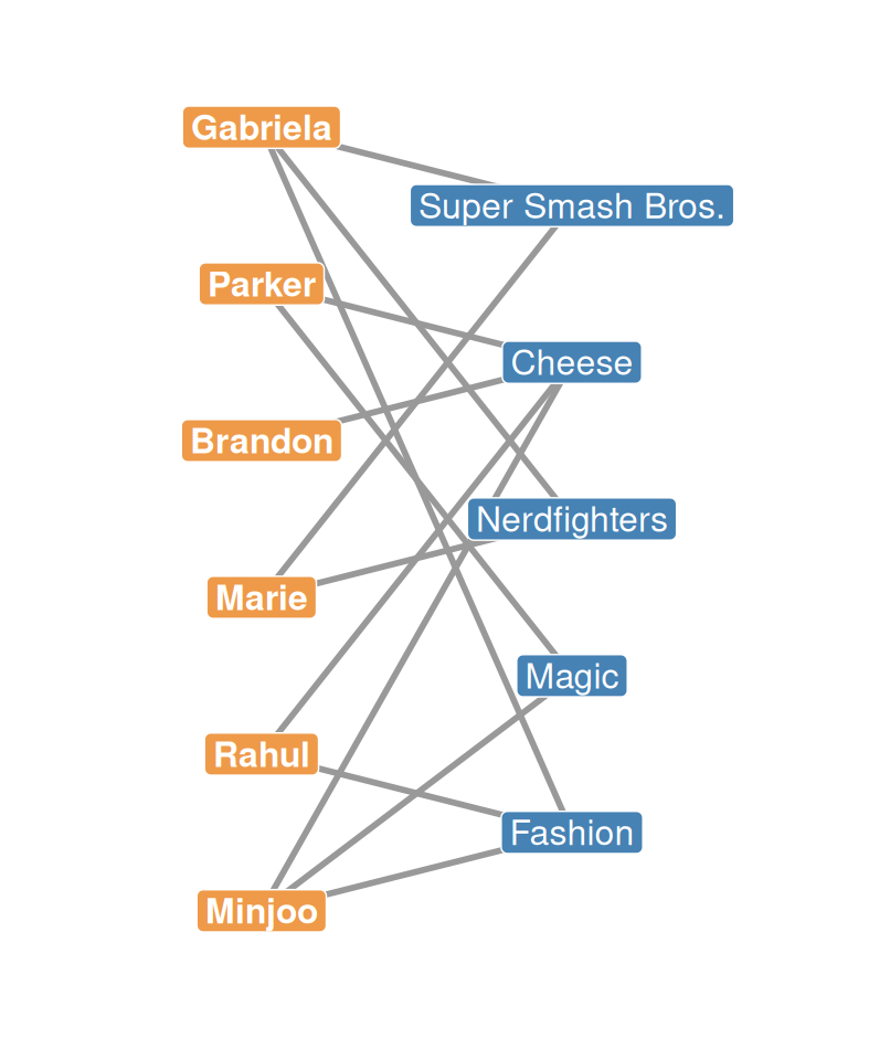
  • Degree works the same way: \(k_i = |N(i)|\)
  • But now there are two sets of degrees, one per mode:

People (\(U\))

Person \(k\)
Gabriela 3
Parker 2
Brandon 1
Marie 2
Rahul 2
Minjoo 3

Groups (\(V\))

Group \(k\)
Super Smash Bros. 2
Cheese 4
Nerdfighters 2
Magic 2
Fashion 3

Graph Metrics Double Up

  • Every degree-based metric now comes in two versions, one per node set:
    • Two degree sequences: \(U = \{3, 3, 2, 2, 2, 1\}\); \(V = \{4, 3, 2, 2, 2\}\)
    • Two maximum/minimum degrees: \(k_{max}(U) = 3\) vs. \(k_{max}(V) = 4\); \(k_{min}(U) = 1\) vs. \(k_{min}(V) = 2\)
    • Two degree ranges: \(k_r(U) = 3 - 1 = 2\); \(k_r(V) = 4 - 2 = 2\)
  • But only one sum of degrees:
    • \(\sum k(U) = 3 + 3 + 2 + 2 + 2 + 1 = 13\)
    • \(\sum k(V) = 4 + 3 + 2 + 2 + 2 = 13\)
    • In a bipartite graph, the sum of the degrees of either node set equals \(m\), the number of edges: \(\sum k(U) = \sum k(V) = m = 13\)

Graph Metrics Double Up (continued)

  • There are still two average degrees, one per mode:
    • \(\bar{k}(U) = 13/|U| = 13/6 \approx 2.2\)
    • \(\bar{k}(V) = 13/|V| = 13/5 = 2.6\)
  • Interpretation:
    • On average, each student belongs to about 2 clubs
    • The average club has about 2–3 members
    • Comparing across modes tells us whether groups are larger than the typical person’s membership portfolio

Part 3: From Bipartite Graph to Affiliation Matrix

Building the Affiliation Matrix

Super Smash Bros. Cheese Nerdfighters Magic Fashion
Gabriela ? ? ? ? ?
Parker ? ? ? ? ?
Brandon ? ? ? ? ?
Marie ? ? ? ? ?
Rahul ? ? ? ? ?
Minjoo ? ? ? ? ?
  • The procedure is the same as for the adjacency matrix of a symmetric graph
  • We build a rectangular matrix \(\mathbf{A}\) of dimensions \(R \times C\):
    • Rows: \(R = |V_1|\) — the people
    • Columns: \(C = |V_2|\) — the groups
  • Cells: \(a_{ij} = 1\) if person \(i\) is affiliated with group \(j\); otherwise \(a_{ij} = 0\)
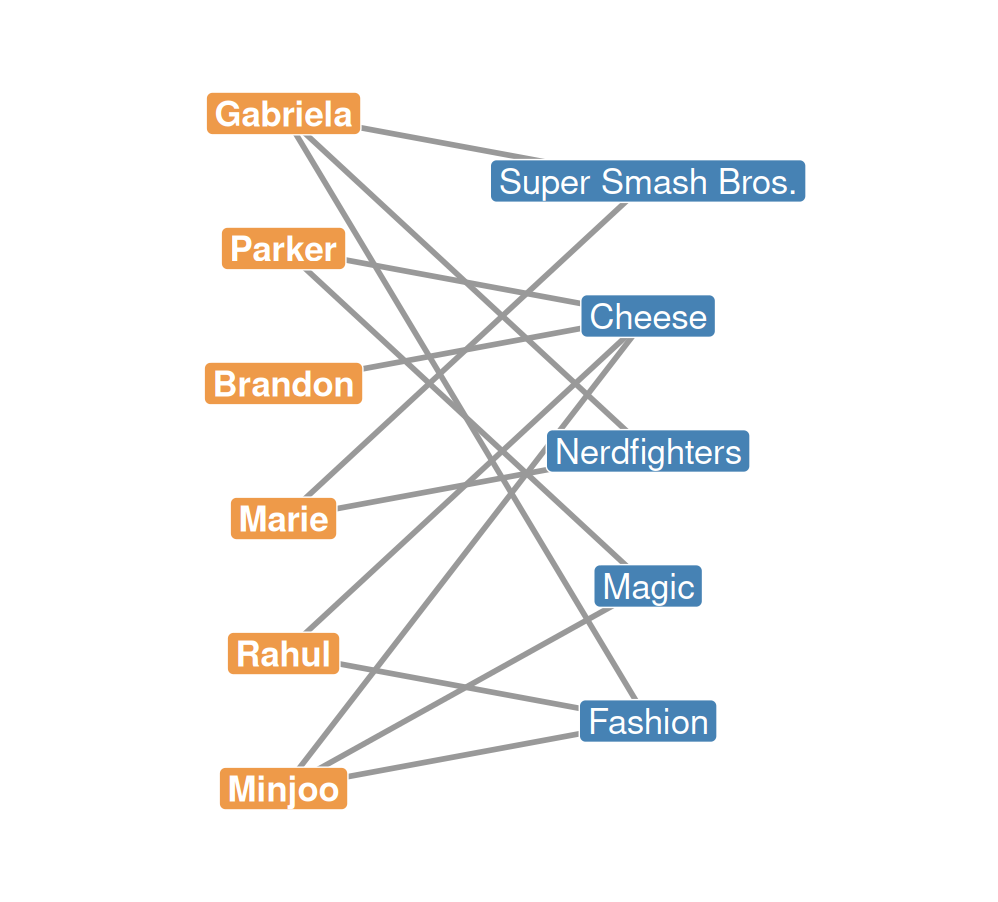
  • We fill it in one row at a time, reading each person’s memberships straight off the graph

Building the Matrix: Gabriela’s Row
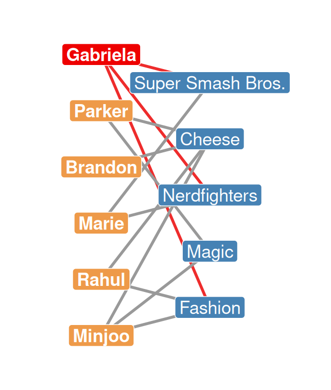
Super Smash Bros. Cheese Nerdfighters Magic Fashion
Gabriela 1 0 1 0 1
Parker ? ? ? ? ?
Brandon ? ? ? ? ?
Marie ? ? ? ? ?
Rahul ? ? ? ? ?
Minjoo ? ? ? ? ?
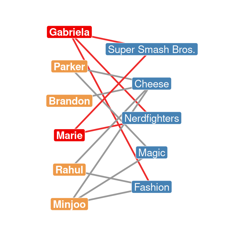
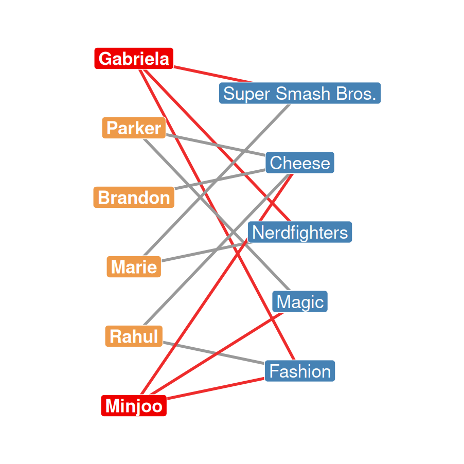
  • Gabriela’s ties (red) point to the Super Smash Bros., Nerdfighters, and Fashion clubs
  • So her row gets a 1 in those three columns, and a 0 everywhere else
  • The zeros are just as informative as the ones: Gabriela does not belong to Cheese or Magic

\[\mathbf{A}_{\text{Gabriela},\cdot} = \color{red}{1}_{SSB} + 0_{Cheese} + \color{red}{1}_{NF} + 0_{Magic} + \color{red}{1}_{Fashion}\]

Building the Matrix: Brandon’s Row
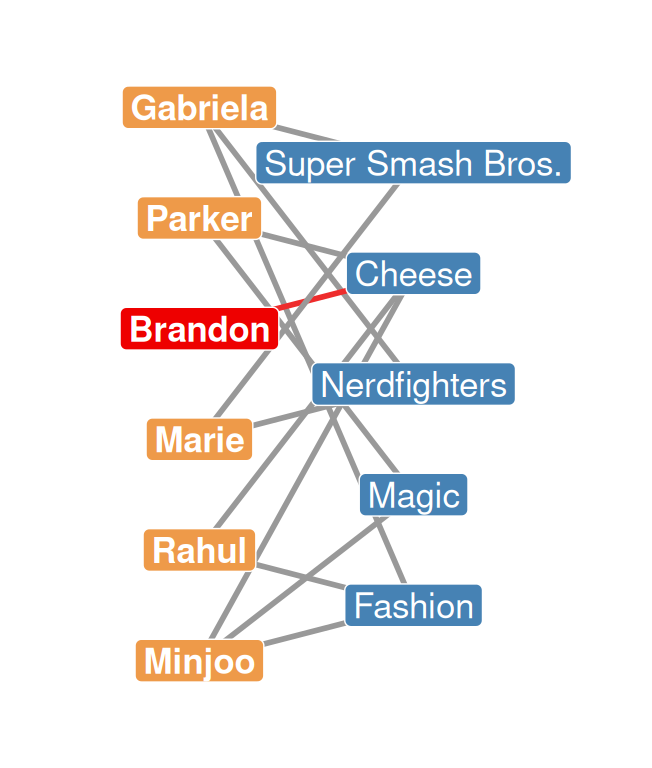
Super Smash Bros. Cheese Nerdfighters Magic Fashion
Gabriela 1 0 1 0 1
Parker ? ? ? ? ?
Brandon 0 1 0 0 0
Marie ? ? ? ? ?
Rahul ? ? ? ? ?
Minjoo ? ? ? ? ?
  • Brandon belongs to exactly one club: the Cheese Club
  • His row therefore contains a single 1 and four 0s
  • Rows can have very different shapes — Gabriela has three memberships, Brandon just one
  • Rows already built (Gabriela, in red) stay in place as we work down the matrix

Building the Matrix: Parker’s Row
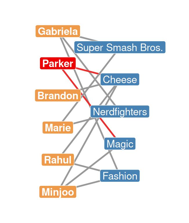
Super Smash Bros. Cheese Nerdfighters Magic Fashion
Gabriela 1 0 1 0 1
Parker 0 1 0 1 0
Brandon 0 1 0 0 0
Marie ? ? ? ? ?
Rahul ? ? ? ? ?
Minjoo ? ? ? ? ?
  • Parker joins the Cheese and Magic clubs: a 1 in each of those columns
  • So far every row has a different pattern: 3, 1, and 2 memberships
  • The same read-the-edges procedure fills every remaining row

The Full Affiliation Matrix

Super Smash Bros. Cheese Nerdfighters Magic Fashion
Gabriela 1 0 1 0 1
Parker 0 1 0 1 0
Brandon 0 1 0 0 0
Marie 1 0 1 0 0
Rahul 0 1 0 0 1
Minjoo 0 1 0 1 1
  • Marie, Rahul, and Minjoo fill in the same way: read the ties, set the matching cells to 1
  • \(\mathbf{A}\) is the affiliation matrix corresponding to the bipartite graph on the right
  • Because the number of people does not have to equal the number of groups, affiliation matrices are usually rectangular, not square like adjacency matrices
Row Sums of the Affiliation Matrix

  • The row sums of the affiliation matrix give the number of memberships each person has: \(C_P^{DEG} = \sum_j a_{ij}\)
Super Smash Bros. Cheese Nerdfighters Magic Fashion Total
Gabriela 1 0 1 0 1 3
Parker 0 1 0 1 0 2
Brandon 0 1 0 0 0 1
Marie 1 0 1 0 0 2
Rahul 0 1 0 0 1 2
Minjoo 0 1 0 1 1 3
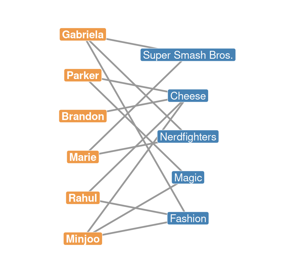
  • Gabriela’s Total (red row) is 3; Brandon’s is just 1 (the Cheese Club) — the degree centrality of the people mode
Column Sums of the Affiliation Matrix

  • The column sums of the affiliation matrix give the size of each group: \(C_G^{DEG} = \sum_i a_{ij}\)
Super Smash Bros. Cheese Nerdfighters Magic Fashion
Gabriela 1 0 1 0 1
Parker 0 1 0 1 0
Brandon 0 1 0 0 0
Marie 1 0 1 0 0
Rahul 0 1 0 0 1
Minjoo 0 1 0 1 1
Total 2 4 2 2 3
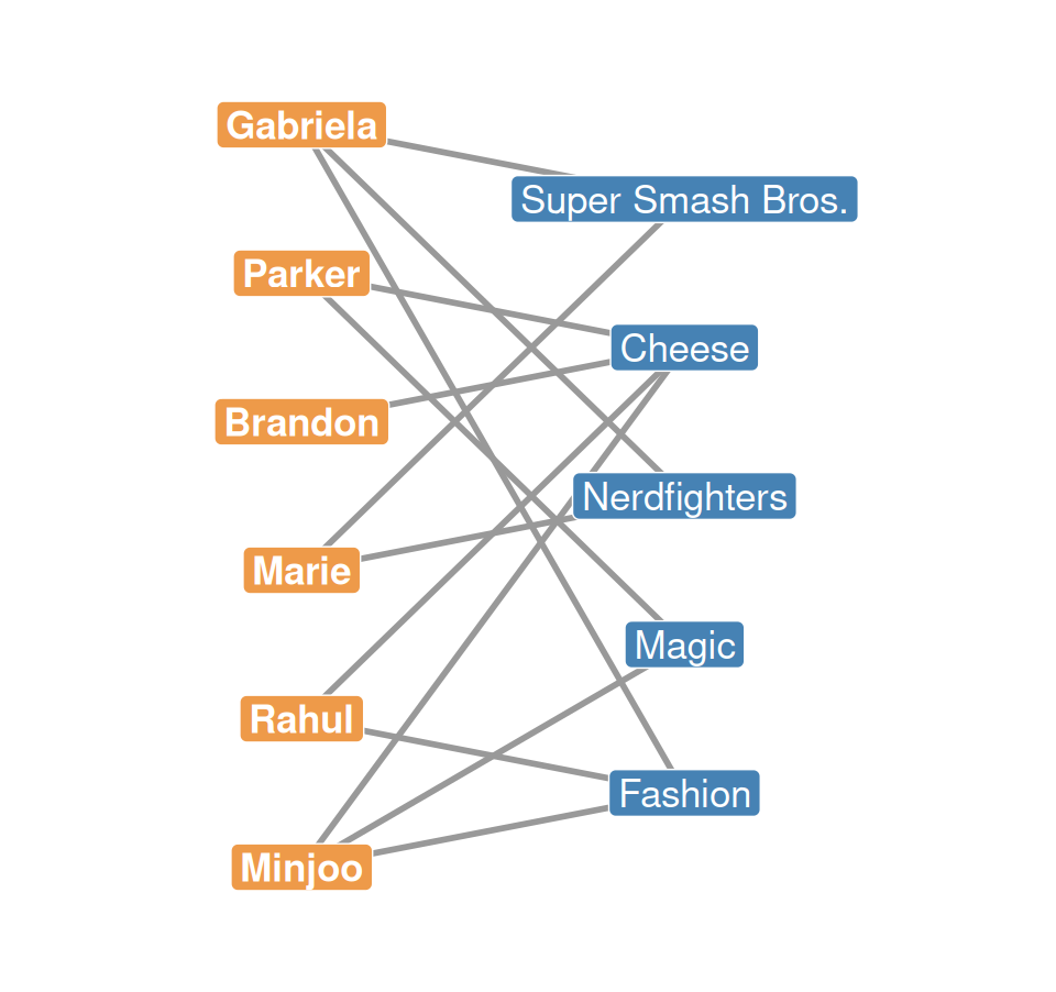
  • The Total row gives each group’s popularity: the Cheese Club (red column) is the most popular (4 members)
  • Two distinct sets of centrality scores — one for the people, one for the groups (Faust 1997)!
Part 4: The Transpose & Matrix Multiplication

The Affiliation Matrix Transpose

\(\mathbf{A}\) (6 × 5)

Super Smash Bros. Cheese Nerdfighters Magic Fashion
Gabriela 1 0 1 0 1
Parker 0 1 0 1 0
Brandon 0 1 0 0 0
Marie 1 0 1 0 0
Rahul 0 1 0 0 1
Minjoo 0 1 0 1 1

\(\mathbf{A}^T\) (5 × 6)

Gabriela Parker Brandon Marie Rahul Minjoo
Super Smash Bros. 1 0 0 1 0 0
Cheese 0 1 1 0 1 1
Nerdfighters 1 0 0 1 0 0
Magic 0 1 0 0 0 1
Fashion 1 0 0 0 1 1
  • The transpose flips rows and columns: \(a^T_{ij} = a_{ji}\)
  • \(\mathbf{A}^T\) contains exactly the same information — but now the groups are in the rows

Matrix Multiplication: Conformability

You can multiply any \(A_{m \times n}\) matrix by any \(B_{q \times p}\) matrix:

\(A_{4 \times 2} \times B_{2 \times 3}\)

  • Inner dimensions match (\(n = q = 2\)): matrices are conformable
  • Result: \(C_{4 \times 3}\) — the outer dimensions

\(A_{4 \times 3} \times B_{2 \times 3}\)

  • Inner dimensions don’t match (\(3 \neq 2\)): matrices are not conformable
  • Product is not defined!
  • The outer dimensions determine the shape of the result: \(A_{m \times n} \times B_{q \times p} = C_{m \times p}\)

Multiplying a Matrix by Its Transpose

  • Turns out the product of any matrix \(\mathbf{A}\) times its transpose \(\mathbf{A}^T\) is always defined!
  • So is the product of the transpose times the original matrix:

\[A_{R \times C} \times A^T_{C \times R} = C_{R \times R}\] \[A^T_{C \times R} \times A_{R \times C} = C_{C \times C}\]

  • The inner dimensions always match (\(C\) vs. \(C\), then \(R\) vs. \(R\))
  • Why do we care? Because these two products extract two new matrices containing not-obvious information about the two-mode network

Part 5: Overlap Matrices

Co-Membership Matrix: Setup

\[O^P = A_{R \times C} \times A^T_{C \times R}\]

  • Multiply the affiliation matrix by its transpose
  • Each cell of the product is the dot product of a row of \(\mathbf{A}\) with a column of \(\mathbf{A}^T\) — but a column of \(\mathbf{A}^T\) is just a row of \(\mathbf{A}\)!

\[o^P_{ij} = \sum_k a_{ik} \, a_{jk}\]

  • \(o^P_{ij}\) counts the clubs \(k\) where both person \(i\) and person \(j\) have a 1 — their shared memberships

Co-Membership Matrix: Worked Example

Super Smash Bros. Cheese Nerdfighters Magic Fashion
Gabriela 1 0 1 0 1
Parker 0 1 0 1 0
Brandon 0 1 0 0 0
Marie 1 0 1 0 0
Rahul 0 1 0 0 1
Minjoo 0 1 0 1 1
  • Red row: Gabriela — fixed in every product
  • Blue rows: the row dotted against her (Marie, then Parker)

Cell (Gabriela, Marie) — Gabriela’s row dotted with Marie’s row:

\[o^P_{GM} = (\color{red}{1})(\color{blue}{1}) + (0)(0) + (\color{red}{1})(\color{blue}{1}) + (0)(0) + (\color{red}{1})(\color{blue}{0}) = \mathbf{2}\]

Cell (Gabriela, Parker):

\[o^P_{GP} = (\color{red}{1})(\color{blue}{0}) + (0)(1) + (\color{red}{1})(\color{blue}{0}) + (0)(1) + (\color{red}{1})(\color{blue}{0}) = \mathbf{0}\]

Cell (Gabriela, Gabriela) — a row dotted with itself:

\[o^P_{GG} = (1)(1) + (0)(0) + (1)(1) + (0)(0) + (1)(1) = \mathbf{3}\]

The Full Co-Membership Matrix

Gabriela Parker Brandon Marie Rahul Minjoo
Gabriela 3 0 0 2 1 1
Parker 0 2 1 0 1 2
Brandon 0 1 1 0 1 1
Marie 2 0 0 2 0 0
Rahul 1 1 1 0 2 2
Minjoo 1 2 1 0 2 3
  • \(O^P = A \times A^T\) transforms the rectangular affiliation matrix into a square matrix with people in both the rows and the columns

Properties of the Co-Membership Matrix

  • Each off-diagonal cell \(o^P_{ij}\): the number of affiliations person \(i\) has in common with person \(j\) (Breiger 1974)
    • Gabriela and Marie share 2 memberships; Gabriela and Parker share none
  • Each diagonal cell \(o^P_{ii}\): the total number of memberships person \(i\) has
    • The diagonal of \(O^P\) is the row-sum vector of \(\mathbf{A}\)!
  • \(O^P\) represents a weighted one-mode network:
    • Strength of tie between \(i\) and \(j\) = number of common memberships
    • A similarity relation — and therefore symmetric

Group Overlap Matrix

\[O^G = A^T_{C \times R} \times A_{R \times C}\]

  • Matrix multiplication is not commutative: \(A \times A^T \neq A^T \times A\) (for rectangular \(\mathbf{A}\)) — so this is a different matrix!
Super Smash Bros. Cheese Nerdfighters Magic Fashion
Super Smash Bros. 2 0 2 0 1
Cheese 0 4 0 2 2
Nerdfighters 2 0 2 0 1
Magic 0 2 0 2 1
Fashion 1 2 1 1 3
  • Off-diagonal cells: the number of members groups \(i\) and \(j\) have in common
  • Diagonal cells: the total number of members in group \(i\) — the column-sum vector of \(\mathbf{A}\)!
  • Super Smash Bros. and Nerdfighters share 2 members; Super Smash Bros. and Cheese share none (a disaffinity!)

Group Overlap Matrix: Worked Example

Gabriela Parker Brandon Marie Rahul Minjoo
Super Smash Bros. 1 0 0 1 0 0
Cheese 0 1 1 0 1 1
Nerdfighters 1 0 0 1 0 0
Magic 0 1 0 0 0 1
Fashion 1 0 0 0 1 1
  • Red row: Super Smash Bros. — fixed in every product
  • Blue rows: the row dotted against it (Nerdfighters, then Cheese)

Cell (SSB, NF) — the Super Smash Bros. row dotted with the Nerdfighters row, matched person by person:

\[o^G_{\text{SSB},\text{NF}} = (\color{red}{1})(\color{blue}{1}) + (0)(0) + (0)(0) + (\color{red}{1})(\color{blue}{1}) + (0)(0) + (0)(0) = \mathbf{2}\]

Cell (SSB, Cheese):

\[o^G_{\text{SSB},\text{Cheese}} = (\color{red}{1})(\color{blue}{0}) + (0)(1) + (0)(1) + (\color{red}{1})(\color{blue}{0}) + (0)(1) + (0)(1) = \mathbf{0}\]

Cell (SSB, SSB) — a row dotted with itself (= group size):

\[o^G_{\text{SSB},\text{SSB}} = (1)(1) + (0)(0) + (0)(0) + (1)(1) + (0)(0) + (0)(0) = \mathbf{2}\]

Overlap = Intersecting Neighborhoods

  • The overlap cell is the cardinality of the intersection of two node neighborhoods:
    • \(N(\text{Gabriela})\) = {Super Smash Bros., Nerdfighters, Fashion}
    • \(N(\text{Marie})\) = {Super Smash Bros., Nerdfighters}

\[\begin{aligned} N(\text{Gabriela}) \cap N(\text{Marie}) &= \{\text{Super Smash Bros.,}\\ &\quad\ \text{Nerdfighters}\} \end{aligned}\]

  • So \(o^P_{\text{Gabriela}, \text{Marie}} = 2\) — exactly what the multiplication computed
  • The same logic works for groups: the group overlap matrix records intersections of member neighborhoods

Part 6: Projections, Duality, and Applications

From Co-Membership Matrix Back to a Graph
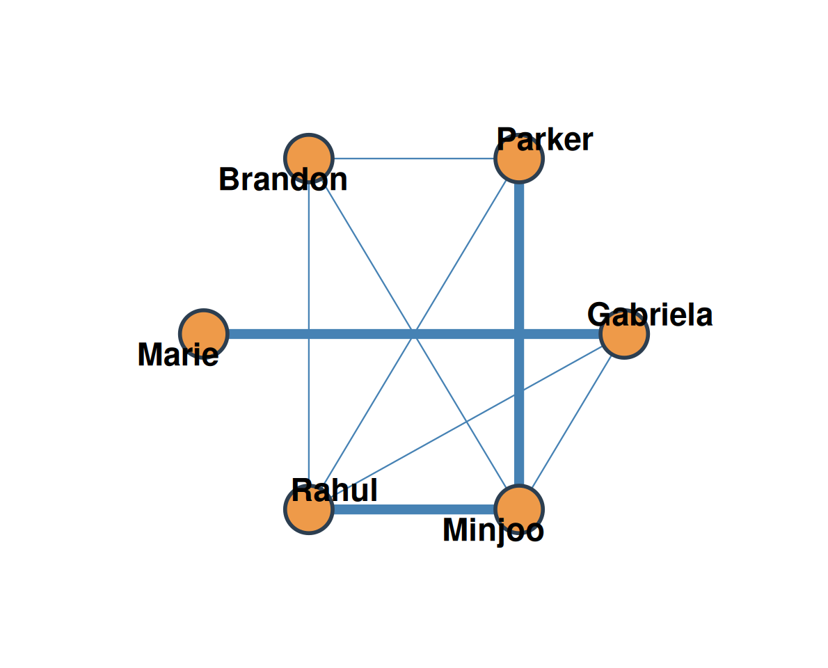
  • \(O^P\) looks like the adjacency matrix of a weighted graph: cells beyond 0/1, symmetric
  • The one-mode (person) projection: ties weighted by the number of shared memberships — a proxy for tie strength when we only have affiliation data

From Group Overlap Matrix Back to a Graph
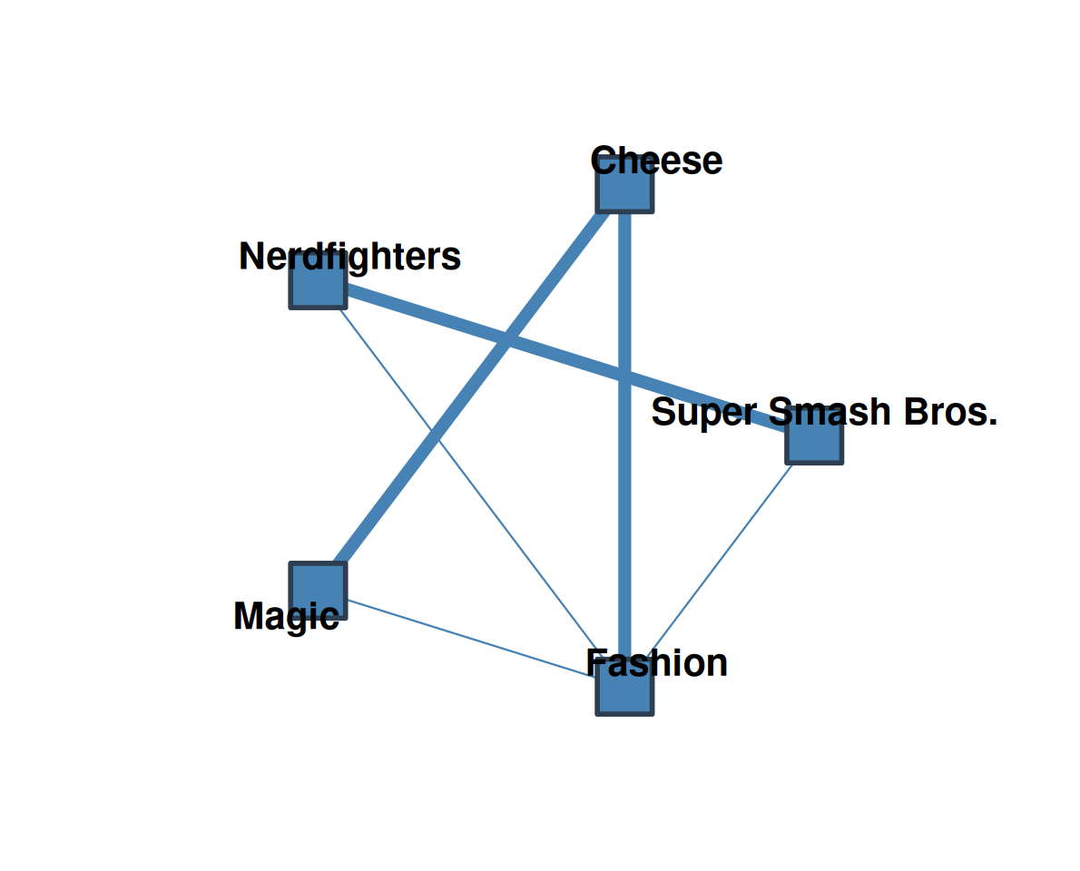
  • The one-mode (group) projection: ties weighted by the number of shared members
  • Super Smash Bros. and Nerdfighters are tightly connected; the Cheese Club is peripheral in the group-to-group network
  • Every two-mode network has two one-mode projections, one per node set

The Duality of Persons and Groups

People are connected to one another by virtue of the groups they belong to; groups are connected to one another by virtue of the people that belong to them. — Breiger (1974)

  • The duality principle: the position of people in a two-mode network is defined by the positions the groups they affiliate with occupy — and vice versa (Bonacich 1991)
  • In our example:
    • Minjoo is peripheral in the person network (few strong ties)
    • The Cheese Club is peripheral in the group network (little overlap with others)
    • Peripheral people belong to peripheral groups!

Application 1: Collaboration Networks

  • In science, the scientist × paper network is an affiliation network
P1 P2 P3 P4 P5 P6
S1 1 1 0 0 1 0
S2 0 0 1 1 0 0
S3 0 1 0 0 0 0
S4 1 0 1 0 0 1
S5 0 1 1 0 0 0
S6 0 1 1 1 1 1
S7 0 0 0 1 0 1
S1 S2 S3 S4 S5 S6 S7
S1 3 0 1 1 1 2 0
S2 0 2 0 1 1 2 1
S3 1 0 1 0 1 1 0
S4 1 1 0 3 1 2 1
S5 1 1 1 1 2 2 0
S6 2 2 1 2 2 5 2
S7 0 1 0 1 0 2 2
  • The co-membership matrix of scientists yields co-authorship teams: \(o^P_{ij}\) = number of papers \(i\) and \(j\) have written together

Application 1: Predicting Future Collaboration
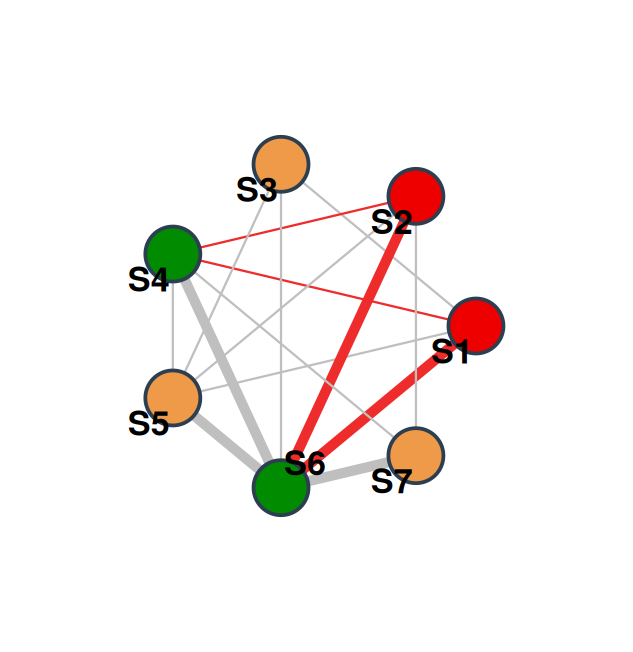
S1 S2 S3 S4 S5 S6 S7
S1 3 0 1 1 1 2 0
S2 0 2 0 1 1 2 1
S3 1 0 1 0 1 1 0
S4 1 1 0 3 1 2 1
S5 1 1 1 1 2 2 0
S6 2 2 1 2 2 5 2
S7 0 1 0 1 0 2 2
  • Red cells: \(o^P_{S4,S6} = 2\) — papers co-authored
  • Blue diagonal: papers written (productivity)
  • The diagonal records productivity: S6 has written 5 papers, S1 and S4 3 each
  • High co-membership = people who know each other and work well together — e.g., S4 and S6 (2 joint papers); S6 has co-authored with everyone
  • So we can predict future collaboration!
    • Repeat collaborators like S4–S6 tend to team up again
    • First ties: S1 and S2 have never co-authored, but the red paths show both working with S4 and S6
    • Mechanism: triadic closure — the shared collaborator who has worked with both brings them onto the next team

Application 2: Product Choice Networks

  • In markets, the person × product network is an affiliation network
  • The overlap matrix gives a product network: movies linked by shared viewers
M1 M2 M3 M4 M5
P1 1 0 0 0 0
P2 1 1 0 0 0
P3 0 0 0 1 1
P4 0 0 1 0 0
P5 1 0 1 0 0
P6 0 0 1 0 0
P7 0 1 0 0 0
P8 0 1 1 0 0
M1 M2 M3 M4 M5
M1 3 1 1 0 0
M2 1 3 1 0 0
M3 1 1 4 0 0
M4 0 0 0 1 1
M5 0 0 0 1 1
  • Movies 1, 2, 3 share watchers — a de facto genre cluster (“rom-coms” vs. “action”)
  • Product networks like this are the basis of recommendation systems — let’s see the process on a graph

Application 2: Recommending Products

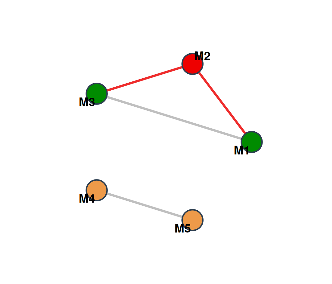
  • Red = the movie a customer just watched (\(M_2\)); green = the recommendations
  • \(M_2\)’s watchers: P2 (also watched \(M_1\)), P7, and P8 (also watched \(M_3\)) — the red ties
  • Nobody who watched \(M_2\) watched \(M_4\) or \(M_5\): no shared watchers, no tie, no recommendation
  • So the system recommends \(M_1\) and \(M_3\): “people who watched \(M_2\) also watched…” is just reading a row of the group overlap matrix — no ratings or genre labels, only co-viewing patterns

Glossary of Key Terms

  • Affiliation network: a social network in which two types of entities (e.g., people and the clubs they join) are linked together
  • Bipartite graph: a graph with two disjoint sets of nodes, in which nodes link only to nodes in the other set
    • Bipartite graphs are the natural representation of two-mode networks!
  • Affiliation matrix: the matrix recording the adjacency relations between vertices in a bipartite graph (people × groups)
  • Matrix transpose: the operation switching the rows and columns of a matrix (\(A_{R \times C} \to A^T_{C \times R}\))
  • Co-membership matrix (\(A \times A^T\)): off-diagonal cells record the number of shared memberships for each pair of people
  • Group overlap matrix (\(A^T \times A\)): off-diagonal cells record the number of shared members for each pair of groups
  • Duality of persons and groups: people’s positions are defined by the groups they belong to; groups’ positions by the people who belong to them (Breiger 1974)

Summary

  • Affiliation networks are two-mode networks: people linked to the groups, events, and projects they join
  • Bipartite graphs represent them; every graph metric doubles up (one version per node set), but \(\sum k(U) = \sum k(V) = m\)
  • The affiliation matrix \(\mathbf{A}\) (people × groups) is rectangular:
    • Row sums = person memberships (degree centrality)
    • Column sums = group sizes (group degree centrality)
  • \(\mathbf{A} \times \mathbf{A}^T\) and \(\mathbf{A}^T \times \mathbf{A}\) are always defined, and yield the co-membership and group overlap matrices — two weighted one-mode projections
  • The duality principle ties it all together: central people belong to central groups
Mizruchi, Mark S. 1983. “Who Controls Whom? An Examination of the Relation Between Management and Boards of Directors in Large American Corporations.” Academy of Management Review 8 (3): 426–35.