| A | B | C | D | E | F | |
|---|---|---|---|---|---|---|
| Row A | 0 | 0 | 1 | 1 | 0 | 0 |
| A - Mean | (0 - 0.33) | (0 - 0.33) | (1 - 0.33) | (1 - 0.33) | (0 - 0.33) | (0 - 0.33) |
| Difference | -0.33 | -0.33 | 0.67 | 0.67 | -0.33 | -0.33 |
Graph Theory: Blockmodeling
Role Structure and Block Relations
Part 1: The Correlation Distance & CONCOR
The Correlation Distance (\(d^{corr}_{k,l}\))
- Beyond Euclidean distance, we can measure structural similarity using the Pearson Correlation Coefficient (\(r_{kl}\) or \(d^{corr}_{kl}\)) between node vectors.
- Compares row (or column) vectors and returns a value between \(-1.0\) and \(+1.0\):
- \(+1.0\): Nodes are perfectly structurally equivalent.
- Positive (\(> 0.0\)): Nodes are structurally similar.
- Negative (\(< 0.0\)): Nodes are structurally dissimilar.
- \(-1.0\): Nodes are completely different, pointing to completely disjoint sets of neighbors.
- The formula is:
- \[d^{corr}_{k, l} = \frac{\sum_j (a_{(k)j} - \overline{a}_{(k)j}) \times (a_{(l)j} - \overline{a}_{(l)j})}{\sqrt{\sum_j (a_{(k)j} - \overline{a}_{(k)j})^2 \times \sum_j (a_{(l)j} - \overline{a}_{(l)j})^2}}\]
Meaning of Row Means (\(\overline{a}_{(k)j}\))
- What does \(\overline{a}_{(k)j}\) represent?
- It is simply the average of the row elements for node \(k\).
- \[\overline{a}_{(k)j} = \frac{\sum_j a_{kj}}{N}\]
- Where \(N\) is the number of columns (the order of the graph).
- For a binary adjacency matrix, the row mean is simply the node degree divided by the number of nodes:
- Node \(A\) has ties to \(\{C, D\}\) in a 6-node network:
- Vector \(a_{(A)j} = (0, 0, 1, 1, 0, 0)\).
- Average: \(\overline{a}_{(A)j} = \frac{2}{6} \approx 0.33\).
Mean Differences Vector
- Subtracting the row mean \(\overline{a}_{(A)j} \approx 0.33\) from each entry of \(A\)’s row vector \(a_{(A)j} = (0, 0, 1, 1, 0, 0)\) gives the Mean Differences vector:
- We compute these difference vectors for all pairs of nodes, multiply them in the numerator, normalize them in the denominator, and obtain the correlation matrix.
Correlation Distance Matrix (\(S^{corr}\))
| A | B | C | D | E | F | |
|---|---|---|---|---|---|---|
| A | -- | 1 | -0.71 | -0.71 | 0.71 | -0.32 |
| B | 1 | -- | -0.71 | -0.71 | 0.71 | -0.32 |
| C | -0.71 | -0.71 | -- | 1 | -1 | 0.45 |
| D | -0.71 | -0.71 | 1 | -- | -1 | 0.45 |
| E | 0.71 | 0.71 | -1 | -1 | -- | -0.45 |
| F | -0.32 | -0.32 | 0.45 | 0.45 | -0.45 | -- |
- Structurally equivalent pairs (\(\{A, B\}\) and \(\{C, D\}\)) have a correlation of 1.00.
- Completely disjoint pairs (\(\{C, E\}\) and \(\{D, E\}\)) are perfectly negatively correlated (-1.00).
- Similar but non-equivalent nodes (\(C\) and \(F\)) have a correlation of 0.45.
Iterated Correlation Distances: CONCOR
- What happens if we take the correlation distance of a correlation distance matrix?
- CONCOR (Convergence of Iterated Correlations; Breiger, Boorman, & Arabie, 1975):
- If we recursively calculate the correlation distance matrix of the previous correlation matrix, the values mathematically converge to only \(+1.0\) and \(-1.0\).
- This slices the network into two distinct, highly clear-cut blocks of structurally equivalent or similar nodes.
- Let’s look at this mathematical convergence in action.
Iterative Convergence (2nd & 3rd Iterations)
2nd Iteration Matrix
- Values begin polarizing toward \(+1\) and \(-1\).
| A | B | C | D | E | F | |
|---|---|---|---|---|---|---|
| A | -- | 1 | -0.97 | -0.97 | 0.97 | -0.84 |
| B | 1 | -- | -0.97 | -0.97 | 0.97 | -0.84 |
| C | -0.97 | -0.97 | -- | 1 | -1 | 0.84 |
| D | -0.97 | -0.97 | 1 | -- | -1 | 0.84 |
| E | 0.97 | 0.97 | -1 | -1 | -- | -0.84 |
| F | -0.84 | -0.84 | 0.84 | 0.84 | -0.84 | -- |
3rd Iteration Matrix
- Every cell reaches exactly \(+1.00\) or \(-1.00\)!
| A | B | C | D | E | F | |
|---|---|---|---|---|---|---|
| A | -- | 1 | -1 | -1 | 1 | -0.99 |
| B | 1 | -- | -1 | -1 | 1 | -0.99 |
| C | -1 | -1 | -- | 1 | -1 | 0.99 |
| D | -1 | -1 | 1 | -- | -1 | 0.99 |
| E | 1 | 1 | -1 | -1 | -- | -0.99 |
| F | -0.99 | -0.99 | 0.99 | 0.99 | -0.99 | -- |
Structural Positions via CONCOR
| A | B | C | D | E | F | |
|---|---|---|---|---|---|---|
| A | 1.00 | 1.00 | -1.00 | -1.00 | 1.00 | -0.99 |
| B | 1.00 | 1.00 | -1.00 | -1.00 | 1.00 | -0.99 |
| C | -1.00 | -1.00 | 1.00 | 1.00 | -1.00 | 0.99 |
| D | -1.00 | -1.00 | 1.00 | 1.00 | -1.00 | 0.99 |
| E | 1.00 | 1.00 | -1.00 | -1.00 | 1.00 | -0.99 |
| F | -0.99 | -0.99 | 0.99 | 0.99 | -0.99 | 1.00 |
- By analyzing the rows of \(+1\) and \(-1\), we extract perfect structurally equivalent positions:
- Position 1 (Salmon): Nodes \(\{A, B\}\)
- Position 2 (Green): Nodes \(\{C, D\}\)
- Position 3 (Blue): Node \(\{E\}\)
- Position 4 (Purple): Node \(\{F\}\)
Part 2: Blockmodeling a 22-Node Network
Uncovering Secret Patterns in Large Networks
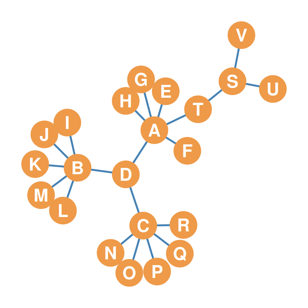
- Let’s apply CONCOR to a larger, messier 22-node network on the right.
- It contains:
- Three high-degree hub nodes (\(A\), \(B\), \(C\)).
- Sets of identical peripheral leaf nodes connected to each hub.
- A highly central node \(D\) bridging hubs.
- Two peripheral nodes \(U, V\) connected only to \(S\).
- Let’s see how CONCOR recursively partitions this graph.
Step 1: First Split (Two Giant Blocks)
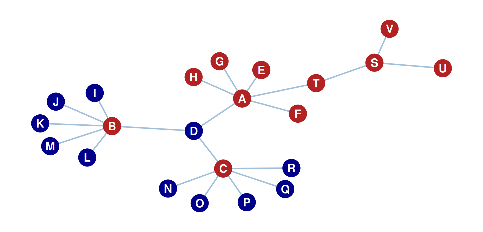
- Running CONCOR on the whole 22-node network splits it into two massive blocks:
- Block 1: \(\{V, U, S, H, G, F, E, T, C, A, B\}\) (Colored Red)
- Block 2: \(\{R, Q, P, O, N, M, L, K, J, D, I\}\) (Colored Blue)
Step 2: Going Deeper (The Hierarchical Partition)
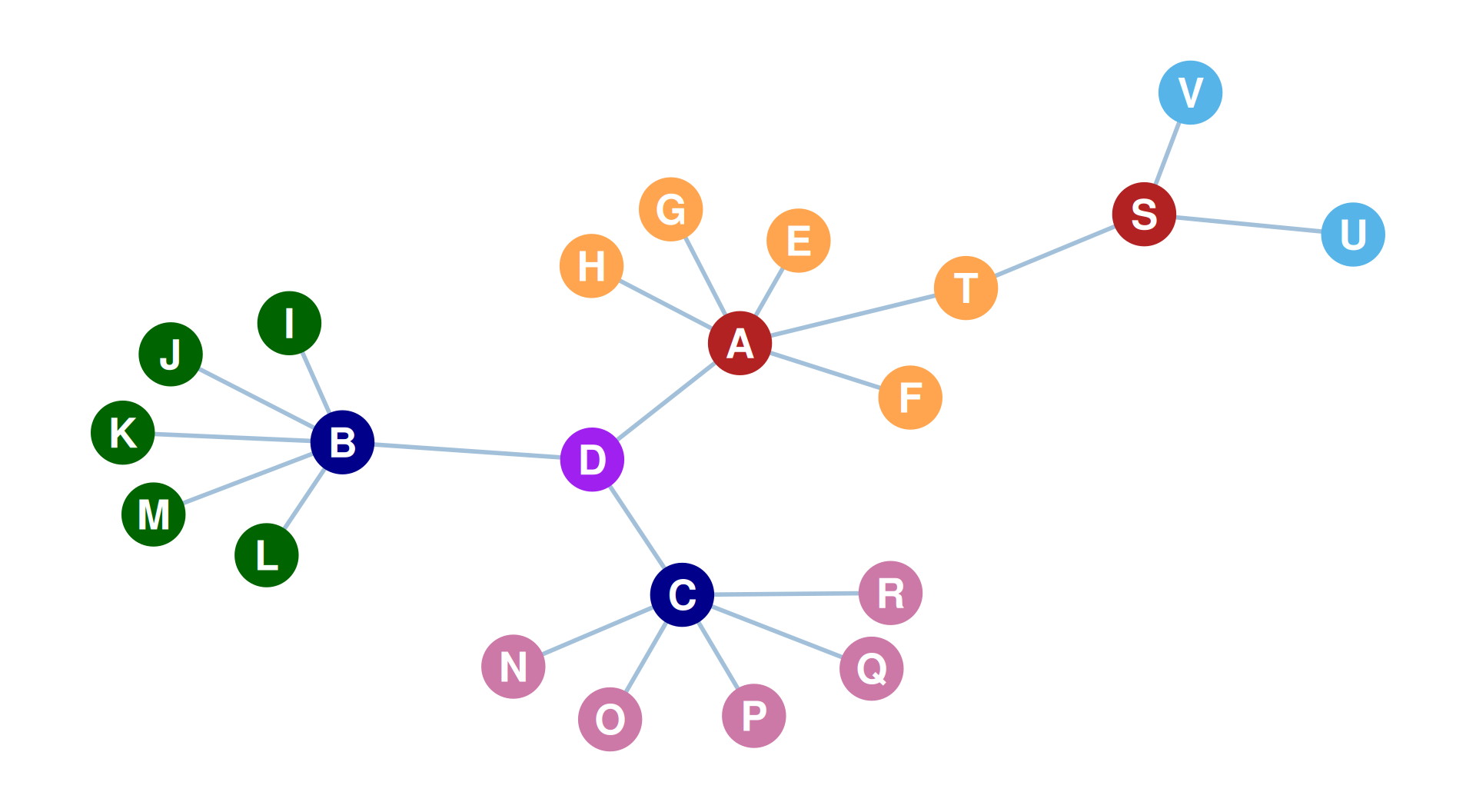
- Running CONCOR recursively on the induced subgraphs of each block yields nested subdivisions:
- Block 1 Splits:
- Block 1a (Core hub/bridge): \(\{A, B, C, S, U, V\}\)
- Block 1b (A’s peripheral leaves): \(\{E, F, G, H, T\}\)
- Block 2 Splits:
- Block 2a (B’s peripheral leaves): \(\{I, J, K, L, M\}\)
- Block 2b (C’s peripheral leaves): \(\{N, O, P, Q, R\}\)
- Block 2c (Unique central bridge): \(\{D\}\) (Occupies a block entirely by itself!)
- Block 1 Splits:
- Further splits on Block 1a isolate \(\{U, V\}\), and divide the remaining \(\{A, B, C, S\}\) into \(\{A, S\}\) and \(\{B, C\}\).
Final Seven-Block Partition
- The final, elegant block partition reveals how role structures are naturally isolated:
The Blocked Adjacency Matrix (Blocks 1–3)
| I | J | K | L | M | N | O | P | Q | R | T | E | F | G | H | B | C | A | S | U | V | D | |
|---|---|---|---|---|---|---|---|---|---|---|---|---|---|---|---|---|---|---|---|---|---|---|
| I | 0 | 0 | 0 | 0 | 0 | 0 | 0 | 0 | 0 | 0 | 0 | 0 | 0 | 0 | 0 | 1 | 0 | 0 | 0 | 0 | 0 | 0 |
| J | 0 | 0 | 0 | 0 | 0 | 0 | 0 | 0 | 0 | 0 | 0 | 0 | 0 | 0 | 0 | 1 | 0 | 0 | 0 | 0 | 0 | 0 |
| K | 0 | 0 | 0 | 0 | 0 | 0 | 0 | 0 | 0 | 0 | 0 | 0 | 0 | 0 | 0 | 1 | 0 | 0 | 0 | 0 | 0 | 0 |
| L | 0 | 0 | 0 | 0 | 0 | 0 | 0 | 0 | 0 | 0 | 0 | 0 | 0 | 0 | 0 | 1 | 0 | 0 | 0 | 0 | 0 | 0 |
| M | 0 | 0 | 0 | 0 | 0 | 0 | 0 | 0 | 0 | 0 | 0 | 0 | 0 | 0 | 0 | 1 | 0 | 0 | 0 | 0 | 0 | 0 |
| N | 0 | 0 | 0 | 0 | 0 | 0 | 0 | 0 | 0 | 0 | 0 | 0 | 0 | 0 | 0 | 0 | 1 | 0 | 0 | 0 | 0 | 0 |
| O | 0 | 0 | 0 | 0 | 0 | 0 | 0 | 0 | 0 | 0 | 0 | 0 | 0 | 0 | 0 | 0 | 1 | 0 | 0 | 0 | 0 | 0 |
| P | 0 | 0 | 0 | 0 | 0 | 0 | 0 | 0 | 0 | 0 | 0 | 0 | 0 | 0 | 0 | 0 | 1 | 0 | 0 | 0 | 0 | 0 |
| Q | 0 | 0 | 0 | 0 | 0 | 0 | 0 | 0 | 0 | 0 | 0 | 0 | 0 | 0 | 0 | 0 | 1 | 0 | 0 | 0 | 0 | 0 |
| R | 0 | 0 | 0 | 0 | 0 | 0 | 0 | 0 | 0 | 0 | 0 | 0 | 0 | 0 | 0 | 0 | 1 | 0 | 0 | 0 | 0 | 0 |
| T | 0 | 0 | 0 | 0 | 0 | 0 | 0 | 0 | 0 | 0 | 0 | 0 | 0 | 0 | 0 | 0 | 0 | 1 | 1 | 0 | 0 | 0 |
| E | 0 | 0 | 0 | 0 | 0 | 0 | 0 | 0 | 0 | 0 | 0 | 0 | 0 | 0 | 0 | 0 | 0 | 1 | 0 | 0 | 0 | 0 |
| F | 0 | 0 | 0 | 0 | 0 | 0 | 0 | 0 | 0 | 0 | 0 | 0 | 0 | 0 | 0 | 0 | 0 | 1 | 0 | 0 | 0 | 0 |
| G | 0 | 0 | 0 | 0 | 0 | 0 | 0 | 0 | 0 | 0 | 0 | 0 | 0 | 0 | 0 | 0 | 0 | 1 | 0 | 0 | 0 | 0 |
| H | 0 | 0 | 0 | 0 | 0 | 0 | 0 | 0 | 0 | 0 | 0 | 0 | 0 | 0 | 0 | 0 | 0 | 1 | 0 | 0 | 0 | 0 |
The Blocked Adjacency Matrix (Blocks 4–7)
| I | J | K | L | M | N | O | P | Q | R | T | E | F | G | H | B | C | A | S | U | V | D | |
|---|---|---|---|---|---|---|---|---|---|---|---|---|---|---|---|---|---|---|---|---|---|---|
| B | 1 | 1 | 1 | 1 | 1 | 0 | 0 | 0 | 0 | 0 | 0 | 0 | 0 | 0 | 0 | 0 | 0 | 0 | 0 | 0 | 0 | 1 |
| C | 0 | 0 | 0 | 0 | 0 | 1 | 1 | 1 | 1 | 1 | 0 | 0 | 0 | 0 | 0 | 0 | 0 | 0 | 0 | 0 | 0 | 1 |
| A | 0 | 0 | 0 | 0 | 0 | 0 | 0 | 0 | 0 | 0 | 1 | 1 | 1 | 1 | 1 | 0 | 0 | 0 | 0 | 0 | 0 | 1 |
| S | 0 | 0 | 0 | 0 | 0 | 0 | 0 | 0 | 0 | 0 | 1 | 0 | 0 | 0 | 0 | 0 | 0 | 0 | 0 | 1 | 1 | 0 |
| U | 0 | 0 | 0 | 0 | 0 | 0 | 0 | 0 | 0 | 0 | 0 | 0 | 0 | 0 | 0 | 0 | 0 | 0 | 1 | 0 | 0 | 0 |
| V | 0 | 0 | 0 | 0 | 0 | 0 | 0 | 0 | 0 | 0 | 0 | 0 | 0 | 0 | 0 | 0 | 0 | 0 | 1 | 0 | 0 | 0 |
| D | 0 | 0 | 0 | 0 | 0 | 0 | 0 | 0 | 0 | 0 | 0 | 0 | 0 | 0 | 0 | 1 | 1 | 1 | 0 | 0 | 0 | 0 |
- Thick black lines divide the matrix into block submatrices.
- Diagonal squares represent within-block ties; off-diagonal rectangles represent between-block ties.
- We identify Zero Blocks (filled only with 0s) and One Blocks (containing some 1s).
Part 3: Image Matrices & Reduced Graphs
Reducing Complexity to an Image Matrix
- The blocked adjacency matrix can be simplified to a reduced image matrix (\(\mathbf{B}\)) of dimensions \(b \times b\) (where \(b = 7\) is the number of blocks).
- Rule of Reduction:
- We record a 0 if the relation block is a Zero Block (completely disconnected).
- We record a 1 if the relation block is a One Block (contains ties).
- This yields a highly simplified map of role interactions:
\[ \mathbf{B} = \begin{pmatrix} \text{Zero} & \text{Zero} & \text{Zero} & \text{One} & \text{Zero} & \text{Zero} & \text{Zero} \\ \text{Zero} & \text{Zero} & \text{Zero} & \text{One} & \text{Zero} & \text{Zero} & \text{Zero} \\ \text{Zero} & \text{Zero} & \text{Zero} & \text{Zero} & \text{One} & \text{Zero} & \text{Zero} \\ \text{One} & \text{One} & \text{Zero} & \text{Zero} & \text{Zero} & \text{Zero} & \text{One} \\ \text{Zero} & \text{Zero} & \text{One} & \text{Zero} & \text{Zero} & \text{One} & \text{One} \\ \text{Zero} & \text{Zero} & \text{Zero} & \text{Zero} & \text{One} & \text{Zero} & \text{Zero} \\ \text{Zero} & \text{Zero} & \text{Zero} & \text{One} & \text{One} & \text{Zero} & \text{Zero} \end{pmatrix} \]
Image Matrix Table
| Leaves_I | Leaves_N | Leaves_T | Hubs_BC | Hubs_AS | Leaves_UV | Bridge_D | |
|---|---|---|---|---|---|---|---|
| Leaves_I | 0 | 0 | 0 | 1 | 0 | 0 | 0 |
| Leaves_N | 0 | 0 | 0 | 1 | 0 | 0 | 0 |
| Leaves_T | 0 | 0 | 0 | 0 | 1 | 0 | 0 |
| Hubs_BC | 1 | 1 | 0 | 0 | 0 | 0 | 1 |
| Hubs_AS | 0 | 0 | 1 | 0 | 0 | 1 | 1 |
| Leaves_UV | 0 | 0 | 0 | 0 | 1 | 0 | 0 |
| Bridge_D | 0 | 0 | 0 | 1 | 1 | 0 | 0 |
- High-level representation of block relations.
- Notice that Leaf blocks do not connect to themselves (0s on diagonal), but connect specifically to their respective Hub blocks.
Reduced Graph Representation
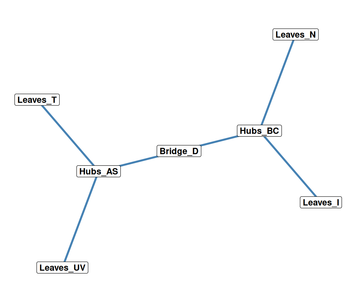
- We can plot the image matrix as a reduced graph.
- The Power of Blockmodeling:
- Distills a sprawling, complex network of 22 nodes down to a highly intuitive role-interaction model of just 7 block-nodes.
- Revealing the structural blueprint of the system: peripheral elements (leaves) feeding into coordinated brokers (hubs), bridged by a highly central node (\(D\)).
Blockmodeling: A Structural Summary
- Blockmodeling Distills Structure:
- Slices complex social structures down to high-level system blueprints.
- CONCOR algorithm:
- Recursively polarizes Pearson correlations to group similar actors.
- Zero vs. One Blocks:
- Blocked adjacency matrices cleanly isolate patterns of connection (One blocks) and absolute separation (Zero blocks).
- Reduced Graph Models:
- Image matrices represent relations between roles, creating simplified reduced graphs that make networks easy to read, interpret, and model.