Centrality in Networks
The Big Three Centrality Metrics: Degree, Closeness, and Betweenness
The Degree Centrality Ranking
| node | score | node | score |
|---|---|---|---|
| j | 7 | l | 3 |
| d | 5 | m | 3 |
| g | 5 | n | 3 |
| b | 4 | p | 3 |
| f | 4 | c | 2 |
| h | 4 | o | 2 |
| i | 4 | q | 2 |
| a | 3 | r | 1 |
| e | 3 | s | 1 |
| k | 3 |
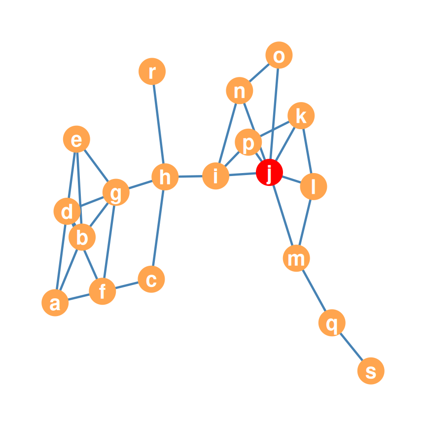
- Node j (7 ties, highlighted) tops the ranking; r and s (1 tie each) sit at the bottom
- Popularity, in graph-theoretic form
Normalized Degree Centrality
- Ranges 0–1: 20 friends is \(\approx 0.02\) in the big school, \(\approx 0.20\) in the small one.
Raw degree is sensitive to network size
Freeman (1979) proposed normalizing by the maximum possible degree, \(N - 1\): \(C_{i(norm)}^{DEG} = C_i^{DEG} / (N - 1)\)
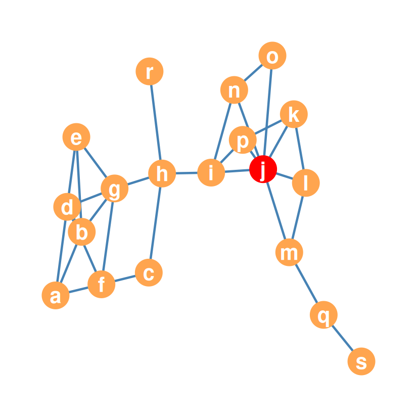
In our example graph, \(N = 19\), so the maximum possible degree is \(N - 1 = 18\)
Example: j scores \(7/18 = 0.39\); r scores \(1/18 = 0.06\) (top and bottom of the table)
| node | score | node | score |
|---|---|---|---|
| j | 0.39 | l | 0.17 |
| d | 0.28 | m | 0.17 |
| g | 0.28 | n | 0.17 |
| b | 0.22 | p | 0.17 |
| f | 0.22 | c | 0.11 |
| h | 0.22 | o | 0.11 |
| i | 0.22 | q | 0.11 |
| a | 0.17 | r | 0.06 |
| e | 0.17 | s | 0.06 |
| k | 0.17 |
The Directed Example
| v1 | v2 | v3 | v4 | v5 | v6 | v7 | v8 | |
|---|---|---|---|---|---|---|---|---|
| v1 | 0 | 1 | 0 | 1 | 0 | 0 | 0 | 0 |
| v2 | 0 | 0 | 1 | 0 | 1 | 0 | 0 | 0 |
| v3 | 1 | 0 | 0 | 1 | 0 | 0 | 0 | 0 |
| v4 | 0 | 0 | 0 | 0 | 1 | 1 | 1 | 0 |
| v5 | 0 | 0 | 1 | 0 | 0 | 0 | 0 | 0 |
| v6 | 0 | 0 | 0 | 0 | 1 | 0 | 0 | 1 |
| v7 | 1 | 0 | 0 | 0 | 0 | 0 | 0 | 0 |
| v8 | 0 | 0 | 0 | 1 | 0 | 0 | 0 | 0 |
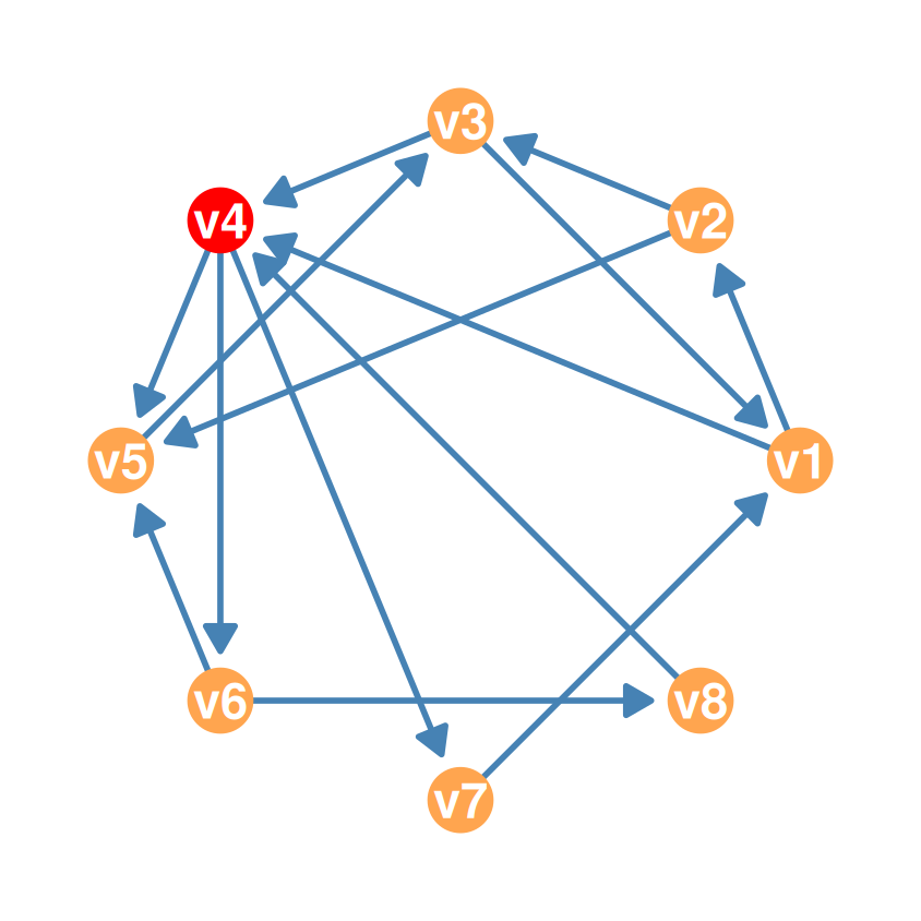
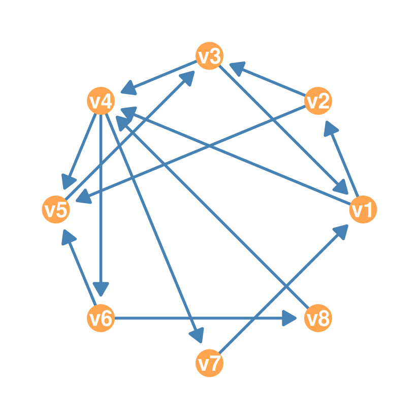
- A strongly connected directed graph: everyone can reach everyone
The Most Closeness-Central Node
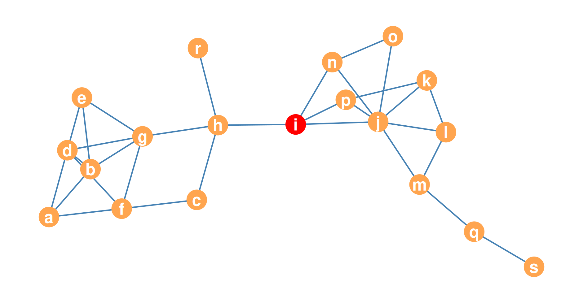
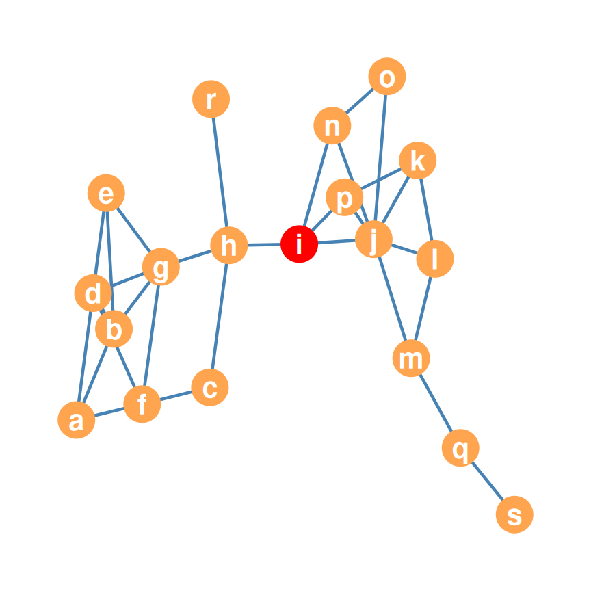
- In this graph, node i has the largest closeness centrality!
Worked Example: Distances from Node i
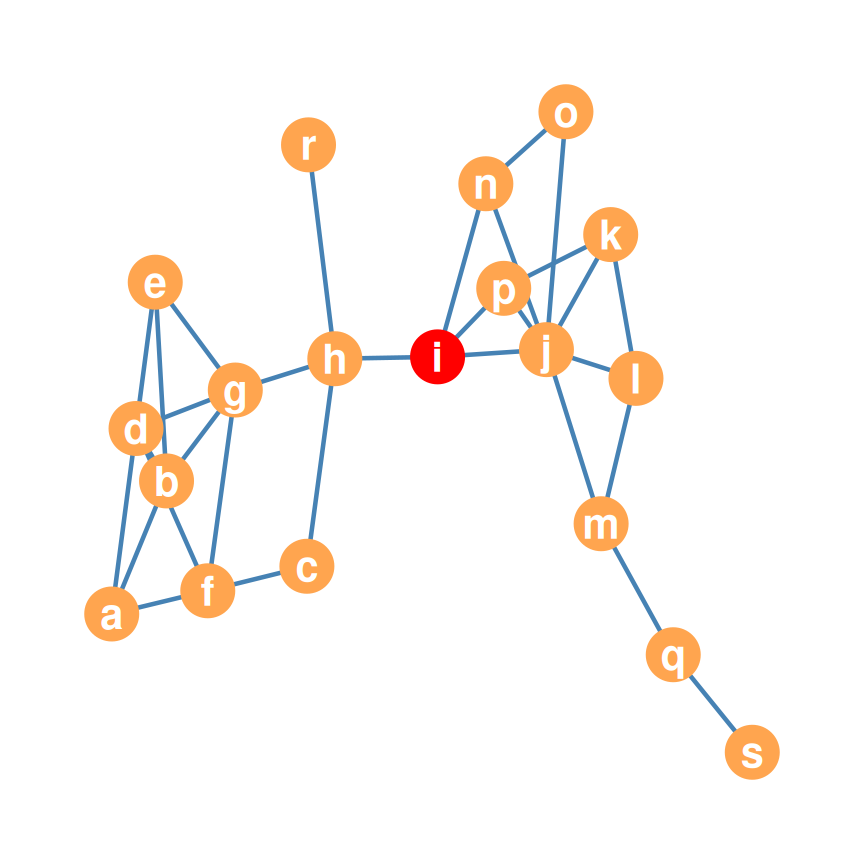
- To compute \(C^{CLOS}(i)\), list the shortest-path distance from i to every other node:
| a | b | c | d | e | f | g | h | i | j | k | l | m | n | o | p | q | r | s |
|---|---|---|---|---|---|---|---|---|---|---|---|---|---|---|---|---|---|---|
| 4 | 3 | 2 | 3 | 3 | 3 | 2 | 1 | 0 | 1 | 2 | 2 | 2 | 1 | 2 | 1 | 3 | 2 | 4 |
\[C^{CLOS}(i) = \frac{N - 1}{\sum_j d_{ij}} = \frac{18}{41} = \mathbf{0.44}\]
Farness: The Row Sums of the Distance Matrix
- Row sums of the distance matrix = total shortest-path distance to all others
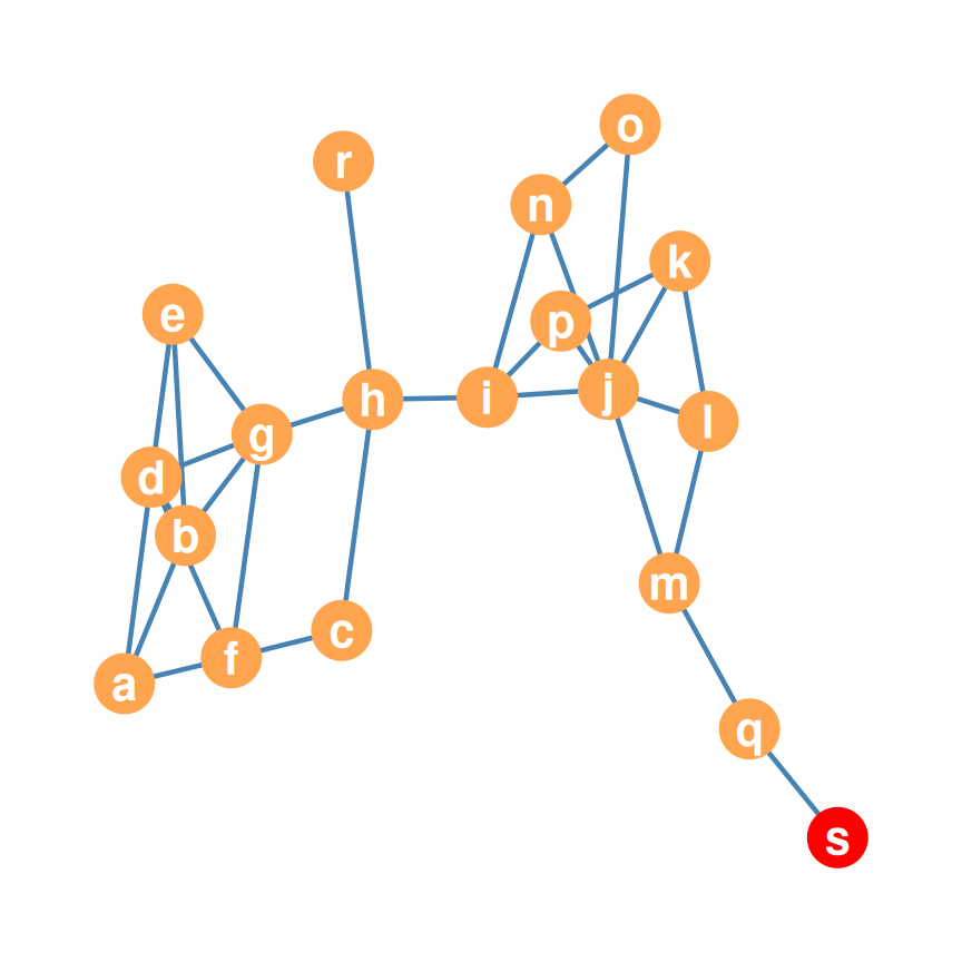
- Bigger = worse: this is farness, not closeness!
| node | farness | node | farness |
|---|---|---|---|
| a | 74 | k | 59 |
| b | 62 | l | 57 |
| c | 54 | m | 56 |
| d | 60 | n | 50 |
| e | 63 | o | 60 |
| f | 61 | p | 50 |
| g | 49 | q | 71 |
| h | 42 | r | 59 |
| i | 41 | s | 88 |
| j | 44 |
- Node s is the most distant node (farness = 88)
From Farness to Closeness
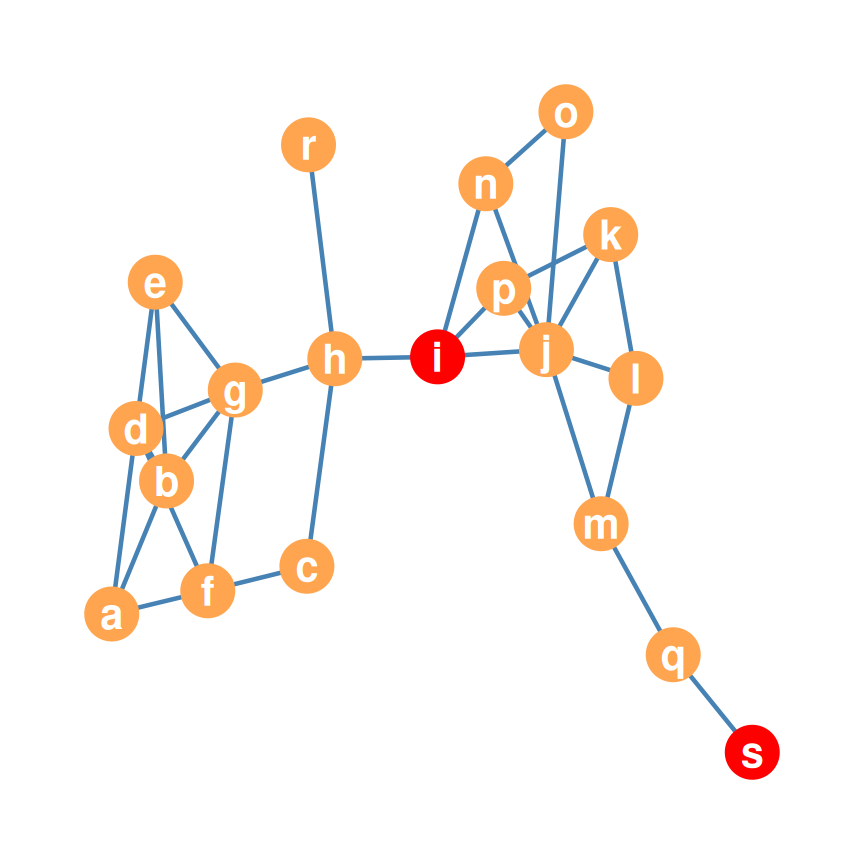
- Ranges 0–1: i tops it (0.44), s sits at the bottom (0.20)
- We want closeness, not farness — so we reverse the scores by dividing \(N - 1\) by each row sum (Freeman 1979): \(C_i^{CLOS} = (N - 1) / \sum_j d_{ij}\)
| node | farness | closeness | node | farness | closeness |
|---|---|---|---|---|---|
| a | 74 | 0.24 | k | 59 | 0.31 |
| b | 62 | 0.29 | l | 57 | 0.32 |
| c | 54 | 0.33 | m | 56 | 0.32 |
| d | 60 | 0.30 | n | 50 | 0.36 |
| e | 63 | 0.29 | o | 60 | 0.3 |
| f | 61 | 0.30 | p | 50 | 0.36 |
| g | 49 | 0.37 | q | 71 | 0.25 |
| h | 42 | 0.43 | r | 59 | 0.31 |
| i | 41 | 0.44 | s | 88 | 0.2 |
| j | 44 | 0.41 |
The Closeness Centrality Ranking
| node | score | node | score |
|---|---|---|---|
| i | 0.44 | r | 0.31 |
| h | 0.43 | d | 0.3 |
| j | 0.41 | f | 0.3 |
| g | 0.37 | o | 0.3 |
| n | 0.36 | b | 0.29 |
| p | 0.36 | e | 0.29 |
| c | 0.33 | q | 0.25 |
| l | 0.32 | a | 0.24 |
| m | 0.32 | s | 0.2 |
| k | 0.31 |
- Node i has the largest closeness centrality (0.44) even though it doesn’t have the largest degree (that was j)!
- Closeness and degree capture different things — the rankings disagree
- Practical use (ch. 19): seed i first to spread an innovation — also the worst node to infect!
Closeness Centrality in Directed Graphs
- Compute closeness in a directed graph as long as the graph is strongly connected — fill up the geodesic distance matrix as usual, starting from the adjacency matrix:
| v1 | v2 | v3 | v4 | v5 | v6 | v7 | v8 | |
|---|---|---|---|---|---|---|---|---|
| v1 | 0 | 1 | 0 | 1 | 0 | 0 | 0 | 0 |
| v2 | 0 | 0 | 1 | 0 | 1 | 0 | 0 | 0 |
| v3 | 1 | 0 | 0 | 1 | 0 | 0 | 0 | 0 |
| v4 | 0 | 0 | 0 | 0 | 1 | 1 | 1 | 0 |
| v5 | 0 | 0 | 1 | 0 | 0 | 0 | 0 | 0 |
| v6 | 0 | 0 | 0 | 0 | 1 | 0 | 0 | 1 |
| v7 | 1 | 0 | 0 | 0 | 0 | 0 | 0 | 0 |
| v8 | 0 | 0 | 0 | 1 | 0 | 0 | 0 | 0 |
The Directed Geodesic Distance Matrix
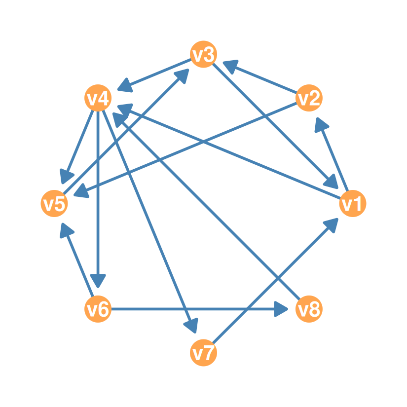
- Filling in shortest-path distances works as usual — except the matrix is now asymmetric!
| v1 | v2 | v3 | v4 | v5 | v6 | v7 | v8 | |
|---|---|---|---|---|---|---|---|---|
| v1 | 0 | 1 | 2 | 1 | 2 | 2 | 2 | 3 |
| v2 | 2 | 0 | 1 | 2 | 1 | 3 | 3 | 4 |
| v3 | 1 | 2 | 0 | 1 | 2 | 2 | 2 | 3 |
| v4 | 2 | 3 | 2 | 0 | 1 | 1 | 1 | 2 |
| v5 | 2 | 3 | 1 | 2 | 0 | 3 | 3 | 4 |
| v6 | 3 | 4 | 2 | 2 | 1 | 0 | 3 | 1 |
| v7 | 1 | 2 | 3 | 2 | 3 | 3 | 0 | 4 |
| v8 | 3 | 4 | 3 | 1 | 2 | 2 | 2 | 0 |
Directed Closeness: Row Sums and Ranking
| node | farness | closeness |
|---|---|---|
| v1 | 13 | 0.54 |
| v2 | 16 | 0.44 |
| v3 | 13 | 0.54 |
| v4 | 12 | 0.58 |
| v5 | 18 | 0.39 |
| v6 | 16 | 0.44 |
| v7 | 18 | 0.39 |
| v8 | 17 | 0.41 |
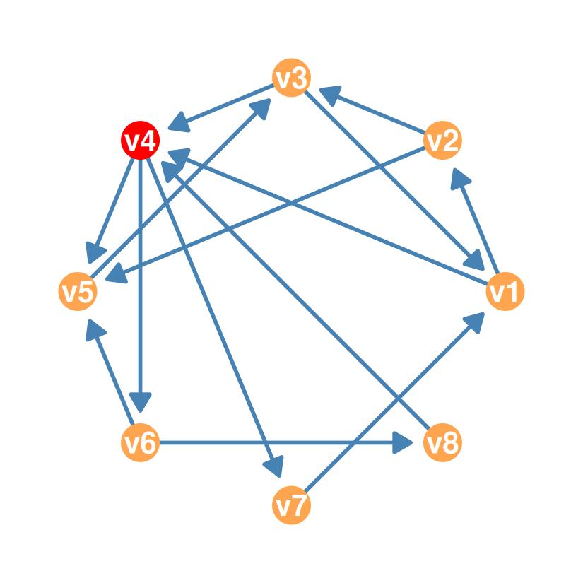
- Node v4 has the largest closeness (0.58) — it is nearest to most nodes
- Note the directionality: v4’s high outdegree and good reach drive this
- Rank order differs from both the outdegree and indegree rankings!
Houston, We Have a Problem
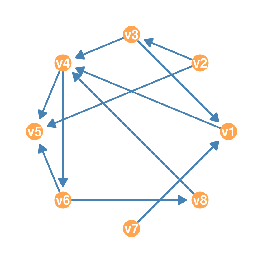
- Now consider a weakly connected directed graph: delete the return ties \(v_1 \to v_2\), \(v_4 \to v_7\), and \(v_5 \to v_3\)
| v1 | v2 | v3 | v4 | v5 | v6 | v7 | v8 | |
|---|---|---|---|---|---|---|---|---|
| v1 | 0 | 0 | 0 | 1 | 0 | 0 | 0 | 0 |
| v2 | 0 | 0 | 1 | 0 | 1 | 0 | 0 | 0 |
| v3 | 1 | 0 | 0 | 1 | 0 | 0 | 0 | 0 |
| v4 | 0 | 0 | 0 | 0 | 1 | 1 | 0 | 0 |
| v5 | 0 | 0 | 0 | 0 | 0 | 0 | 0 | 0 |
| v6 | 0 | 0 | 0 | 0 | 1 | 0 | 0 | 1 |
| v7 | 1 | 0 | 0 | 0 | 0 | 0 | 0 | 0 |
| v8 | 0 | 0 | 0 | 1 | 0 | 0 | 0 | 0 |
- No one can reach nodes v2 and v7 (pure transmitters)
- Node v5 can reach no one (pure receiver)
The Row Sums Turn to Infinity
| v1 | v2 | v3 | v4 | v5 | v6 | v7 | v8 | |
|---|---|---|---|---|---|---|---|---|
| v1 | 0 | Inf | Inf | 1 | 2 | 2 | Inf | 3 |
| v2 | 2 | 0 | 1 | 2 | 1 | 3 | Inf | 4 |
| v3 | 1 | Inf | 0 | 1 | 2 | 2 | Inf | 3 |
| v4 | Inf | Inf | Inf | 0 | 1 | 1 | Inf | 2 |
| v5 | Inf | Inf | Inf | Inf | 0 | Inf | Inf | Inf |
| v6 | Inf | Inf | Inf | 2 | 1 | 0 | Inf | 1 |
| v7 | 1 | Inf | Inf | 2 | 3 | 3 | 0 | 4 |
| v8 | Inf | Inf | Inf | 1 | 2 | 2 | Inf | 0 |
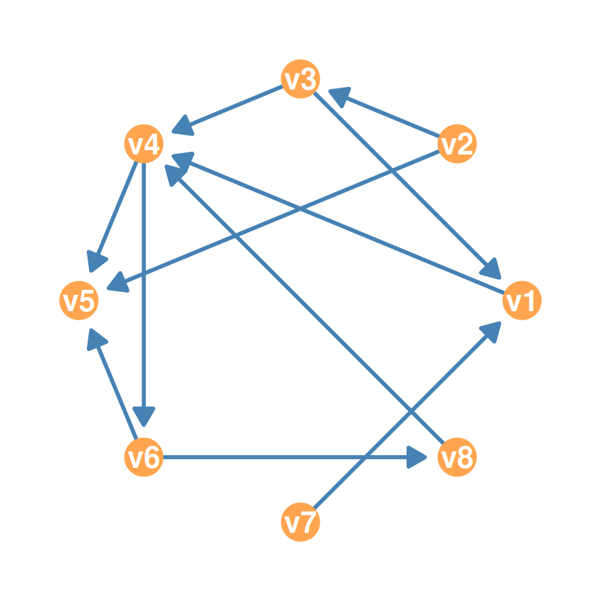
- The geodesic distance between some pairs is now infinity — and the row sums turn into Infs: for any number \(x\), \(x + \infty = \infty\)
- Closeness is undefined!
The Harmonic Centrality Ranking
| node | harmonic | normalized |
|---|---|---|
| v2 | 3.58 | 0.51 |
| v3 | 3.33 | 0.48 |
| v4 | 2.50 | 0.36 |
| v6 | 2.50 | 0.36 |
| v7 | 2.42 | 0.35 |
| v1 | 2.33 | 0.33 |
| v8 | 2.00 | 0.29 |
| v5 | 0.00 | 0.00 |
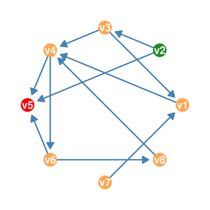
- v2 (green) is now highest (0.51): even though nobody can reach it, it can reach almost everybody quickly
- v5 (red) gets exactly 0: it can reach no one at all
- Harmonic centrality is defined for all graphs — connected or not!
Betweenness Centrality
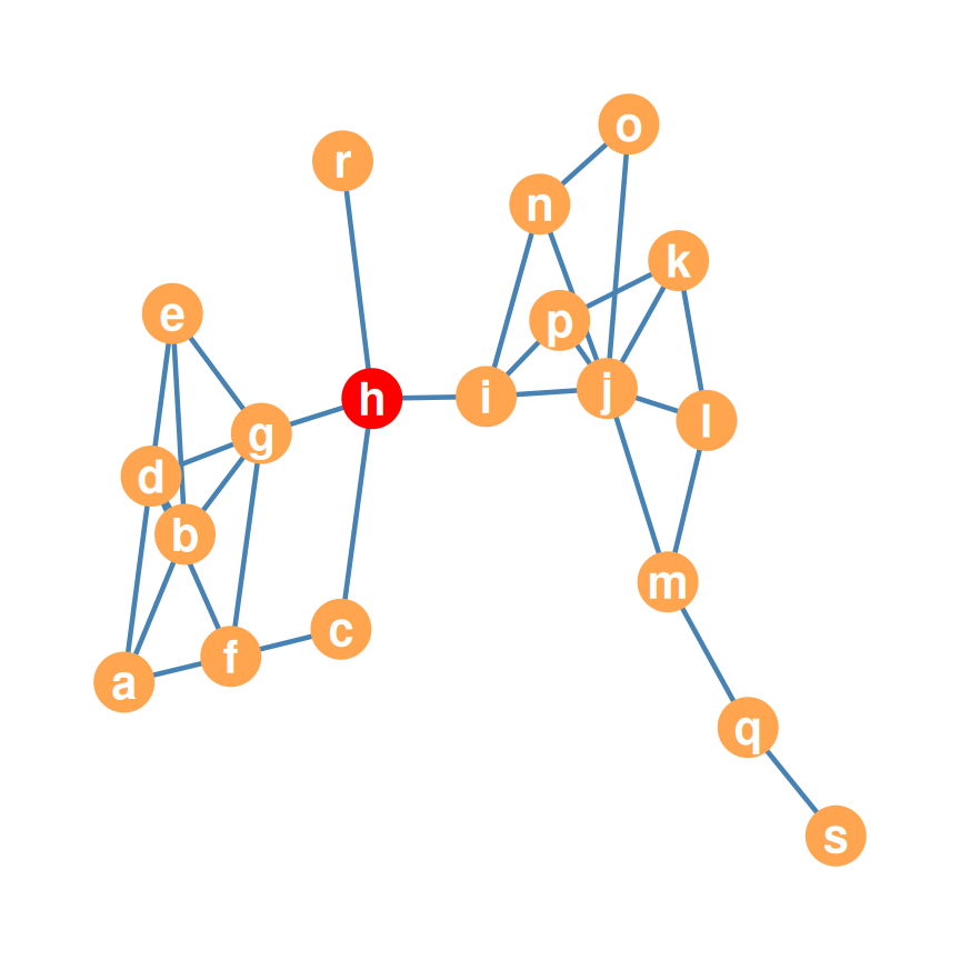
- Betweenness centrality asks: how often does a node sit in the middle of shortest paths connecting other pairs of nodes?
- Picture messages, rumors, or goods traveling from node to node along shortest paths
- A high-betweenness node is a middleperson: a large share of those trips pass straight through it
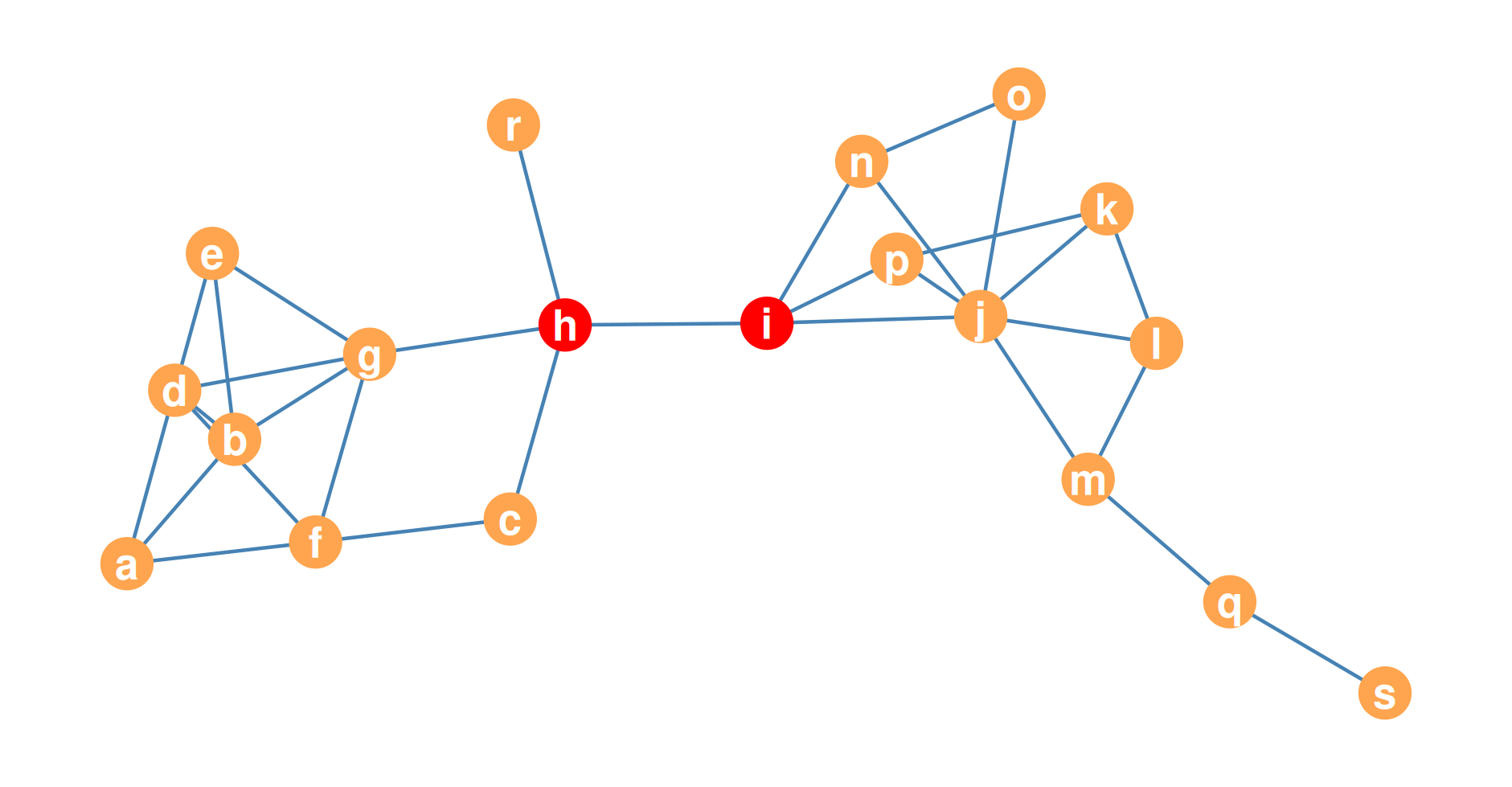
- In our 19-node graph, node h stands on the shortest path between g and i: \(g \to h \to i\)
- Also on the shortest paths between p and c, and between k and r
- h must have high betweenness: it connects the nodes on the left of the graph with the nodes on the right
- Node g is also high-betweenness — but not as high as h!
What is an “Inner Node”?
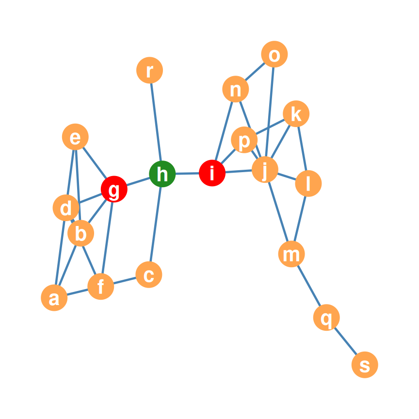
- Pick any two other nodes — say g and i (the red endpoints)
- This graph has exactly one shortest path between them: \(g \to h \to i\)
- h is the inner node — the middleperson (green)
- Every trip between g and i passes through h: \(p_{g(h)i} = 1\) — a full point for h!
- Betweenness: collect h’s share for every pair of other nodes, then add it all up
Stress Centrality: A First Attempt
- A first attempt at betweenness: for each node \(k\), count how many shortest paths between every other pair \(i, j\) feature \(k\) as an inner node — the total traffic through \(k\) (Shimbel 1953): \(C^{STRESS}_k = \sum_{i \neq k} \sum_{j \neq k} n_{i(k)j}\)
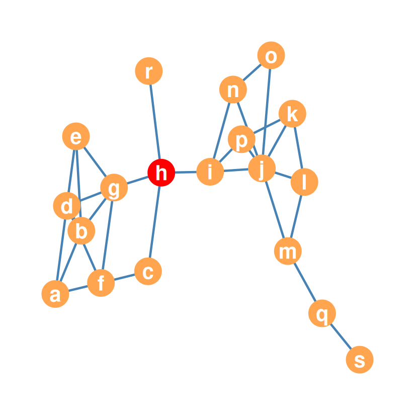
| node | stress | node | stress |
|---|---|---|---|
| a | 4 | k | 2 |
| b | 32 | l | 6 |
| c | 56 | m | 84 |
| d | 40 | n | 28 |
| e | 0 | o | 0 |
| f | 74 | p | 28 |
| g | 208 | q | 44 |
| h | 316 | r | 0 |
| i | 288 | s | 0 |
| j | 206 |
Relative Betweenness: A Worked Example
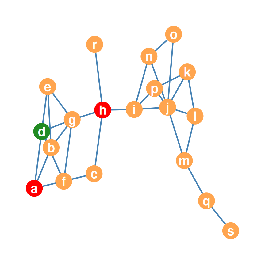
- The relative betweenness of \(k\) w.r.t. nodes \(i, j\) = the proportion of shortest paths between \(i\) and \(j\) that feature \(k\) as an inner node
- What is \(d\)’s relative betweenness w.r.t. \(h\) and \(a\)? (endpoints in red; the candidate inner node d in green)
First, list all shortest paths between h and a:
- \(\{h, g, d, a\}\) — d is on this path!
- \(\{h, c, f, a\}\) — d is not
- \(\{h, g, b, a\}\) — d is not
- \(\{h, g, f, a\}\) — d is not
- So \(d\) appears on 1 out of 4 shortest paths: \(p_{h(d)a} = \frac{1}{4} = \mathbf{0.25}\)
- Interpretation: a random \(h\)-to-\(a\) shortest path has a 25% chance of going through \(d\)
The Betweenness Centrality Ranking
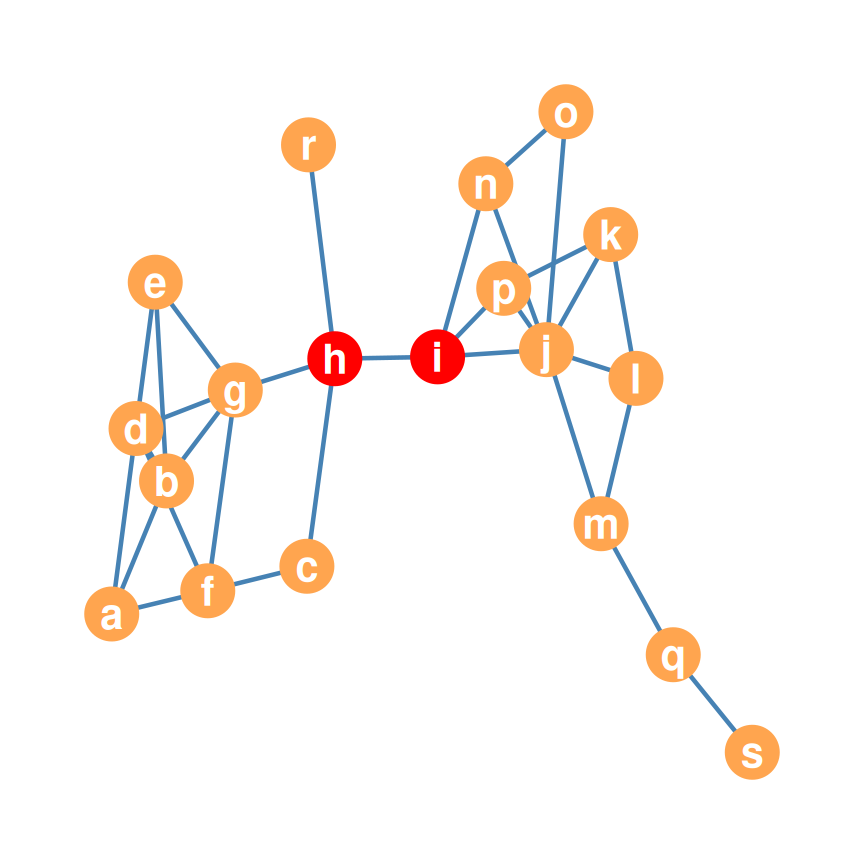
| node | score | node | score |
|---|---|---|---|
| h | 88.1 | p | 5 |
| i | 81.5 | b | 3.8 |
| j | 66.5 | l | 1.5 |
| g | 53.0 | a | 0.6 |
| m | 32.0 | k | 0.5 |
| q | 17.0 | e | 0 |
| f | 10.2 | o | 0 |
| c | 9.0 | r | 0 |
| d | 5.2 | s | 0 |
| n | 5.0 |
- h and i are the top betweenness nodes — they broker between the left and right halves of the graph
- e, o, r, and s have betweenness zero: they don’t stand on any shortest paths between any pair of other nodes
- Closeness = reachability; betweenness = intermediation — different winners!
The Star Graph
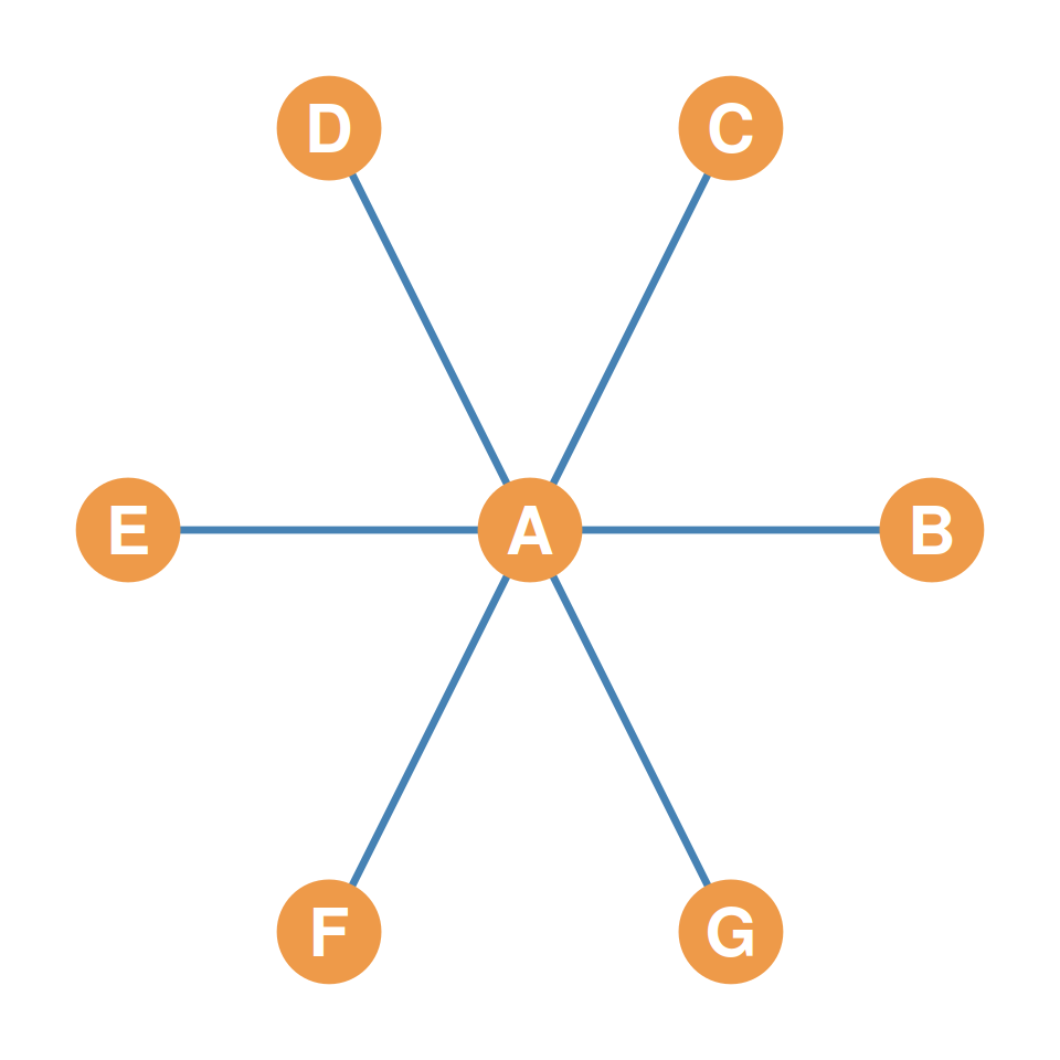
- One central node (A) connected to all \(n - 1\) satellite nodes (B–G); satellites connect to nobody else
- Edge count: \(m = n - 1\)
The Big Three in the Star Graph
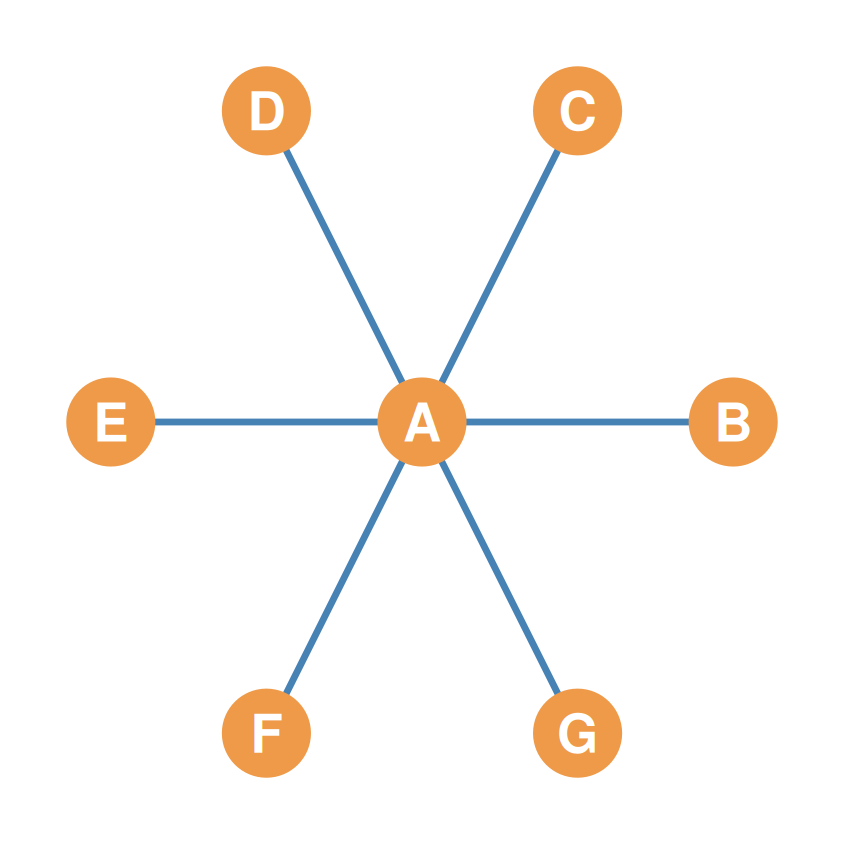
- In the star graph, all three centralities are maximized for the central node (Freeman 1979):
| A | B | C | D | E | F | G | |
|---|---|---|---|---|---|---|---|
| node | A | B | C | D | E | F | G |
| degree | 6 | 1 | 1 | 1 | 1 | 1 | 1 |
| closeness | 1.00 | 0.55 | 0.55 | 0.55 | 0.55 | 0.55 | 0.55 |
| betweenness | 15 | 0 | 0 | 0 | 0 | 0 | 0 |
- Degree: the central node has \(n - 1\); every satellite just 1
- Closeness: the center reaches everyone via paths of length 1; satellites need length 2 to reach each other
- Betweenness: the center stands on every shortest path linking satellite pairs (all length 2)
- That’s why these three are the “big three”: they are precisely the metrics maximized at the center of a star
Centralization of the Star: The Maximum
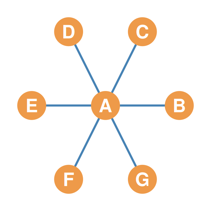
- Take the 7-node star: \(k_{max} = 6\)
- Center A falls short by \(6 - 6 = 0\)
- Each of the six satellites falls short by \(6 - 1 = 5\)
- Sum of shortfalls: \(0 + 6 \times 5 = \mathbf{30}\)
- Benchmark: \((n-1)(n-2) = 6 \times 5 = \mathbf{30}\)
- Degree centralization \(= 30/30 = \mathbf{1.00}\) — the maximum!
- The star is the most centralized graph of its size
Graph Degree Centralization: Worked Example
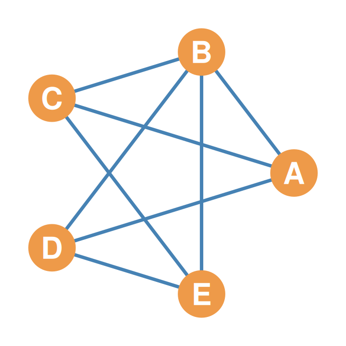
| node | k | diff |
|---|---|---|
| A | 3 | 1 |
| B | 4 | 0 |
| C | 3 | 1 |
| D | 3 | 1 |
| E | 3 | 1 |
- Sum of differences: \(1 + 0 + 1 + 1 + 1 = \mathbf{4}\)
- Star of the same order: \((n-1)(n-2) = 4 \times 3 = \mathbf{12}\)
- Degree centralization \(= 4/12 = \mathbf{0.33}\)
The Other Extreme: The Complete Graph
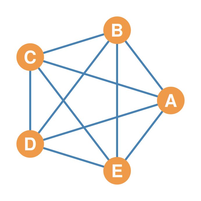
- In the complete graph on 5 nodes, everyone ties: \(k_{max} = 4\) and every \(k_i = 4\)
- Every shortfall: \(4 - 4 = 0\); sum of shortfalls: \(\mathbf{0}\)
- Degree centralization \(= 0/12 = \mathbf{0.00}\) — the minimum!
- Our 19-node example lands in between: \(71/306 = 0.23\)
- Centralization: how unevenly centrality is distributed across the whole graph — 0 (egalitarian) to 1 (star)