Measuring Ego Networks
Ego Network Metrics: Size, Effective Size, Composition, Homophily, Diversity, and Clustering
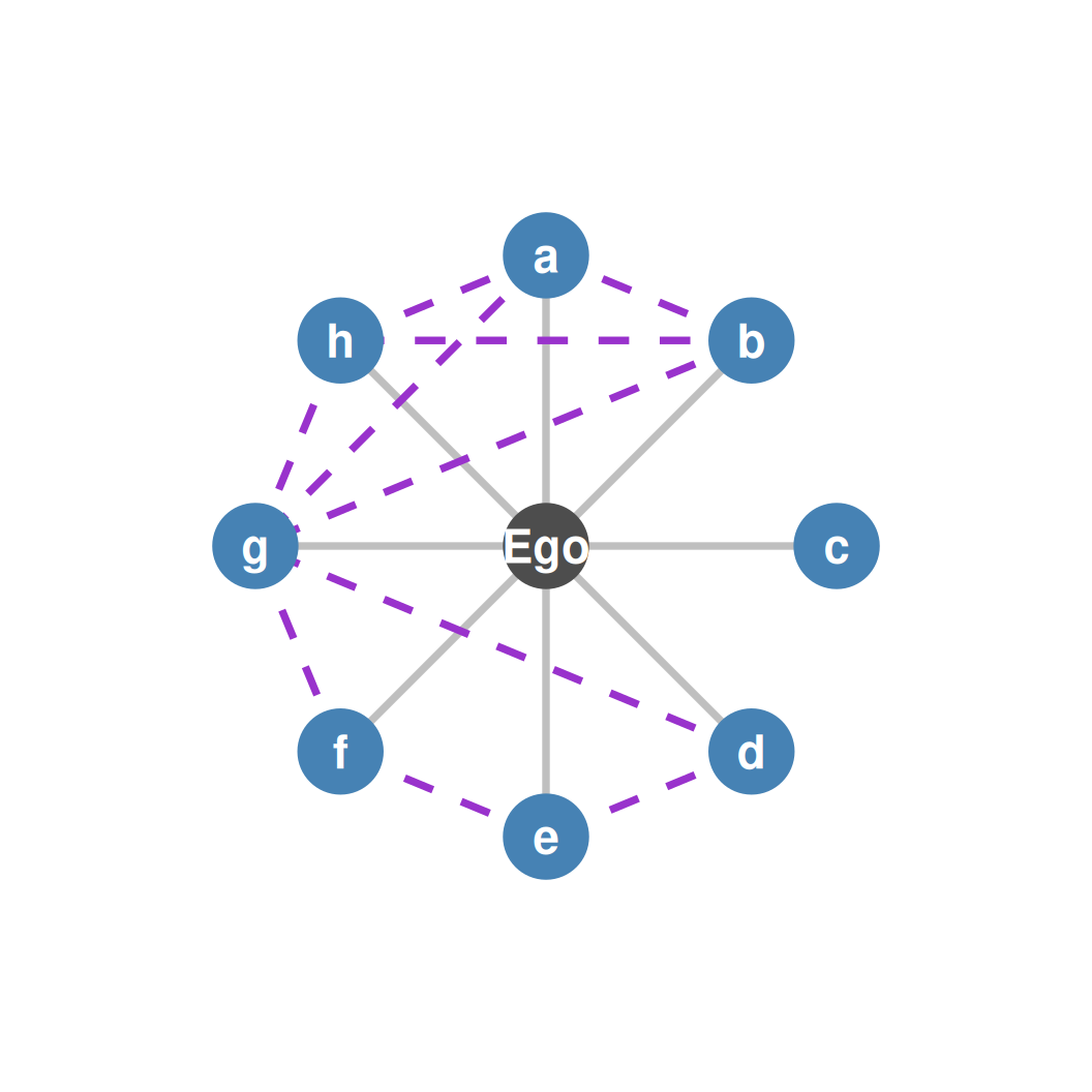
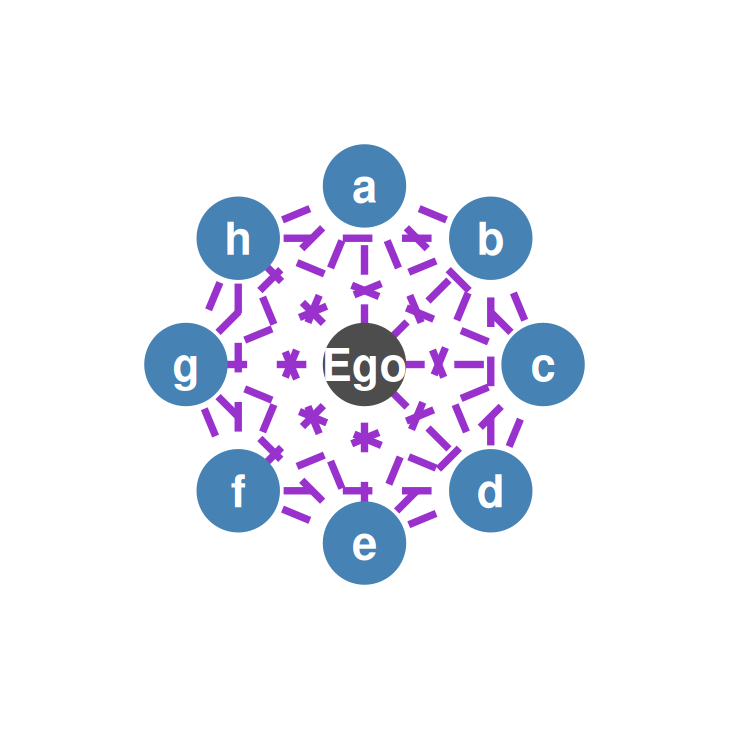
The Two Subgraphs of an Ego Network
- The star subgraph contains all the ego-to-alter ties (\(E_{ea}\)).
- The alter-alter subgraph is the local network among the people who are connected to ego.
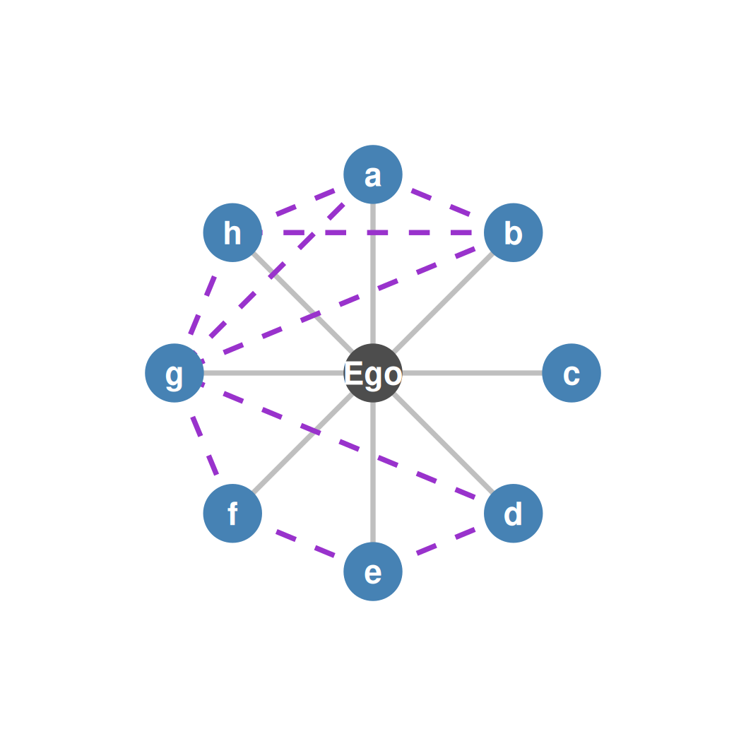
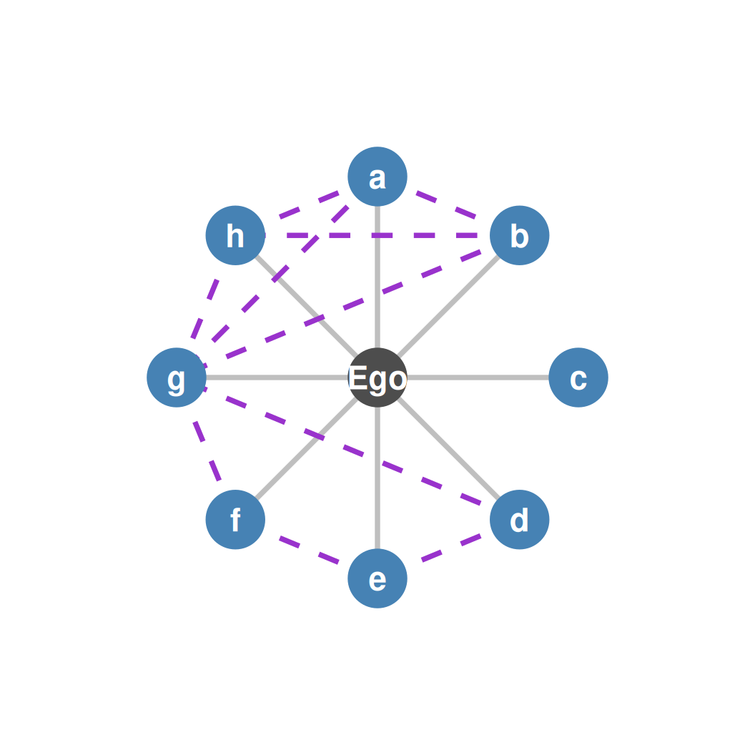
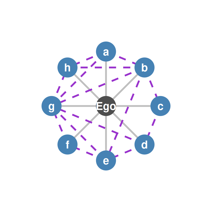
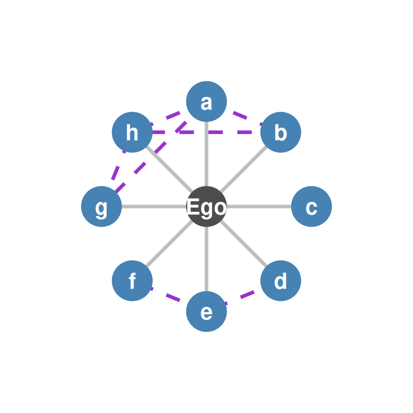
- Alter set: \(V = \{a, b, c, d, e, f, g, h\}\)
- Alter-alter ties: \(E = \{ab, ah, ag, bh, bg, de, dg, ef, fg, gh\}\)
Ego Network Data: What You Need
There are four pieces of information we need to compute the basic ego-network properties:
- The number of ego-alter ties — the same as the number of alters!
- The number of alter-alter ties.
- Sociodemographic characteristics of ego: age, gender, racial identity, class, education.
- Sociodemographic characteristics of alters: the same attributes, for each alter.
Size
- Tells us whether your ego network is large or small — the number of alters (equivalently, ego-alter ties).
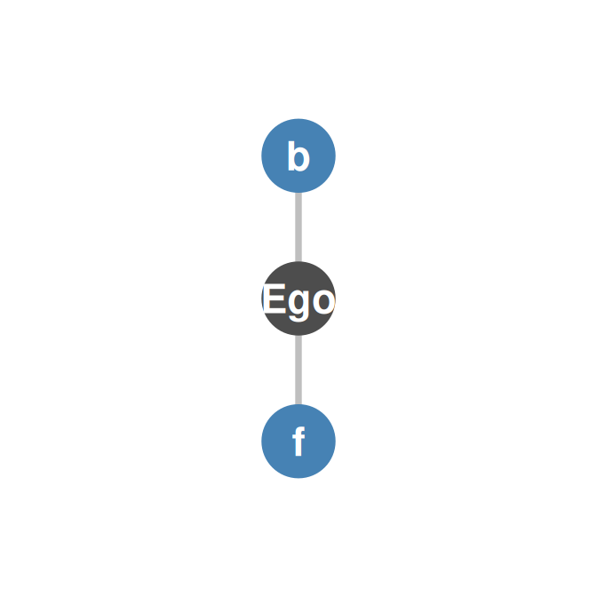
Small: Size = 2
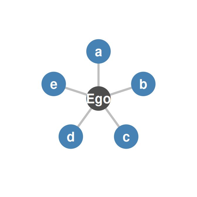
Medium: Size = 5
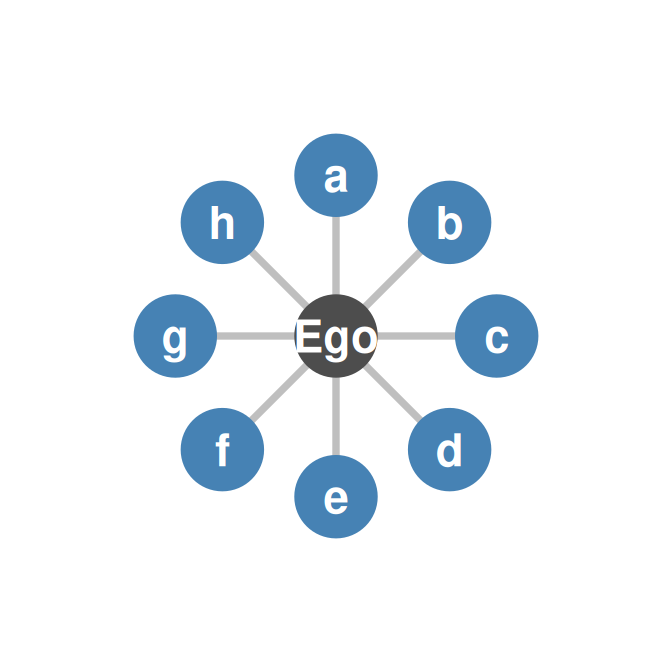
Large: Size = 8
Effective Size: The Idea
- Still tells us whether your ego network is large or small.
- But discounts alters who are connected to one another as redundant.
- Given by ego-network size minus the average degree of the alter-alter subgraph:
\[ES = S - \frac{2m}{n}\]
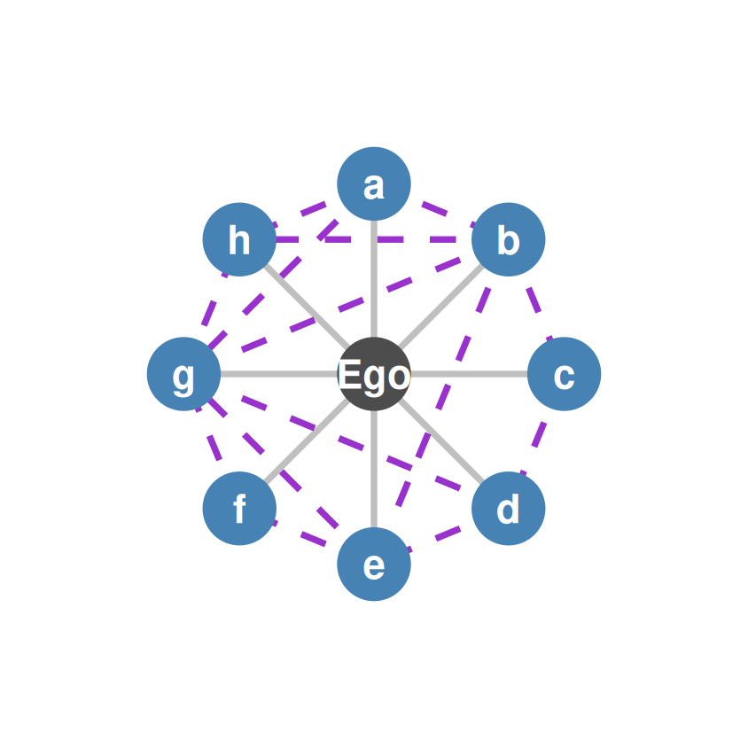
Effective Size: A Dense Alter-Alter Network
| a | b | c | d | e | f | g | h | |
|---|---|---|---|---|---|---|---|---|
| a | 0 | 1 | 0 | 0 | 0 | 0 | 1 | 1 |
| b | 1 | 0 | 1 | 0 | 1 | 0 | 1 | 1 |
| c | 0 | 1 | 0 | 1 | 0 | 0 | 0 | 0 |
| d | 0 | 0 | 1 | 0 | 1 | 0 | 1 | 0 |
| e | 0 | 1 | 0 | 1 | 0 | 1 | 1 | 0 |
| f | 0 | 0 | 0 | 0 | 1 | 0 | 1 | 0 |
| g | 1 | 1 | 0 | 1 | 1 | 1 | 0 | 1 |
| h | 1 | 1 | 0 | 0 | 0 | 0 | 1 | 0 |
- \(n = 8\) alters; \(m = 14\) ties. Each tie appears twice in the matrix (above and below the diagonal); the shaded 1s count each tie once: \(m = 28/2 = 14\).
\[ES = 8 - \frac{28}{8} = 8 - 3.5 = 4.5\]
Effective Size: A Sparse Alter-Alter Network
| a | b | c | d | e | f | g | h | |
|---|---|---|---|---|---|---|---|---|
| a | 0 | 1 | 0 | 0 | 0 | 0 | 1 | 1 |
| b | 1 | 0 | 0 | 0 | 0 | 0 | 0 | 1 |
| c | 0 | 0 | 0 | 0 | 0 | 0 | 0 | 0 |
| d | 0 | 0 | 0 | 0 | 1 | 0 | 0 | 0 |
| e | 0 | 0 | 0 | 1 | 0 | 1 | 0 | 0 |
| f | 0 | 0 | 0 | 0 | 1 | 0 | 0 | 0 |
| g | 1 | 0 | 0 | 0 | 0 | 0 | 0 | 1 |
| h | 1 | 1 | 0 | 0 | 0 | 0 | 1 | 0 |
- The shaded 1s give \(m = 14/2 = 7\). Same size (\(S = 8\)), but less redundancy: the sparse network has the larger effective size.
\[ES = 8 - \frac{14}{8} = 8 - 1.75 = 6.25\]
Effective Size: The Maximum
| a | b | c | d | e | f | g | h | |
|---|---|---|---|---|---|---|---|---|
| a | 0 | 0 | 0 | 0 | 0 | 0 | 0 | 0 |
| b | 0 | 0 | 0 | 0 | 0 | 0 | 0 | 0 |
| c | 0 | 0 | 0 | 0 | 0 | 0 | 0 | 0 |
| d | 0 | 0 | 0 | 0 | 0 | 0 | 0 | 0 |
| e | 0 | 0 | 0 | 0 | 0 | 0 | 0 | 0 |
| f | 0 | 0 | 0 | 0 | 0 | 0 | 0 | 0 |
| g | 0 | 0 | 0 | 0 | 0 | 0 | 0 | 0 |
| h | 0 | 0 | 0 | 0 | 0 | 0 | 0 | 0 |
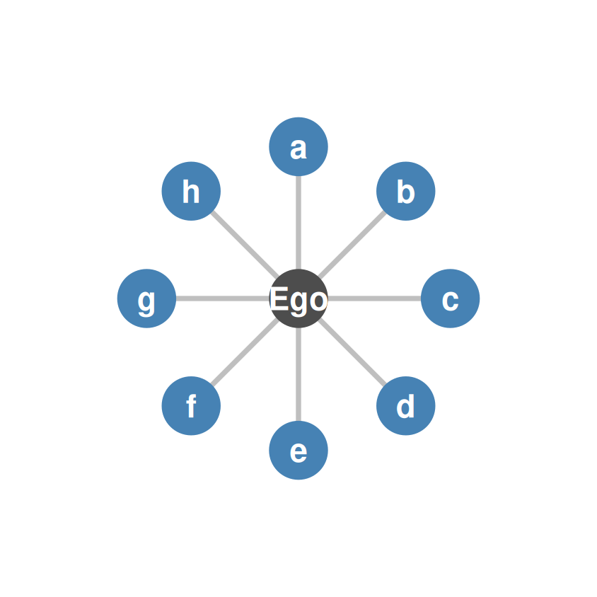
- No alter-alter ties at all (\(m = 0\)): a pure star. No alter is redundant, so nothing gets discounted.
\[ES = 8 - \frac{0}{8} = 8 = S\]
Effective Size: The Minimum
| a | b | c | d | e | f | g | h | |
|---|---|---|---|---|---|---|---|---|
| a | 0 | 1 | 1 | 1 | 1 | 1 | 1 | 1 |
| b | 1 | 0 | 1 | 1 | 1 | 1 | 1 | 1 |
| c | 1 | 1 | 0 | 1 | 1 | 1 | 1 | 1 |
| d | 1 | 1 | 1 | 0 | 1 | 1 | 1 | 1 |
| e | 1 | 1 | 1 | 1 | 0 | 1 | 1 | 1 |
| f | 1 | 1 | 1 | 1 | 1 | 0 | 1 | 1 |
| g | 1 | 1 | 1 | 1 | 1 | 1 | 0 | 1 |
| h | 1 | 1 | 1 | 1 | 1 | 1 | 1 | 0 |
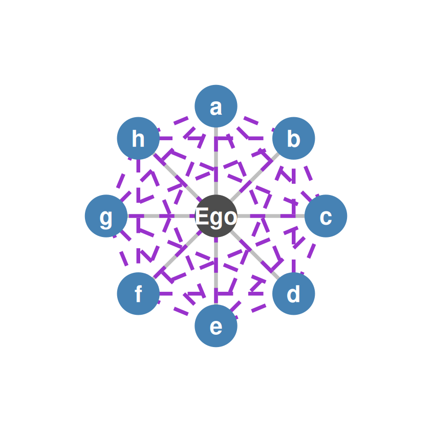
- Every alter knows every other (\(m = 28 = \binom{8}{2}\)): all alters are mutually redundant, so the whole circle acts like a single effective contact.
\[ES = 8 - \frac{56}{8} = 8 - 7 = 1\]
Composition
- Tells us whether your ego network is dominated by one category of alters.
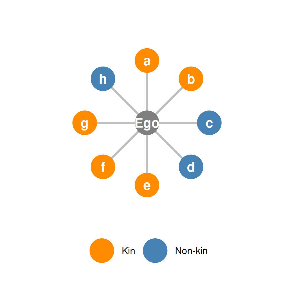
- Given by the proportion of alters who belong to a category: kin, friends, neighbors, co-workers; gender, race, education.
\[Prop(Kin) = \frac{\text{number of kin alters}}{S}\]
- Here: \(Prop(Kin) = 5/8 = 0.63\) — a kin-heavy ego network.
Composition: Another Example
- Composition can be computed for any category the alters fall into.
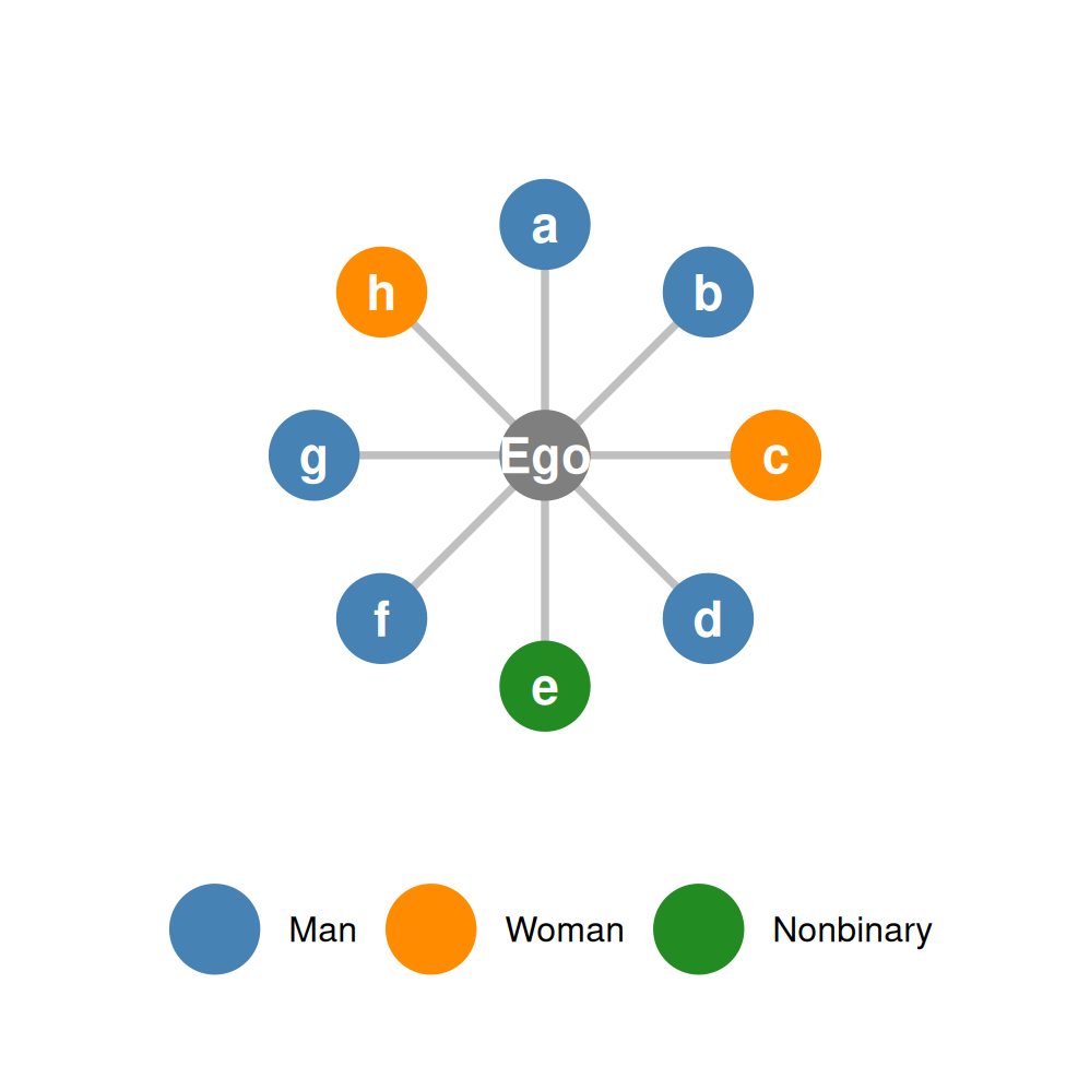
The same network by gender identity:
- \(Prop(Men) = 5/8 = 0.63\)
- \(Prop(Women) = 2/8 = 0.25\)
- \(Prop(Nonbinary) = 1/8 \approx 0.13\)
- Same take: the network is predominantly male.
Homophily: The E-I Index
- Tells us whether the people in your ego network are the same or different from you on some sociodemographic characteristic: age, race, gender, education.
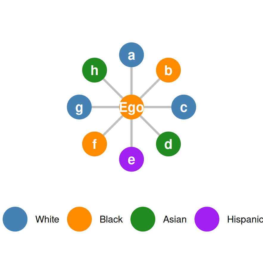
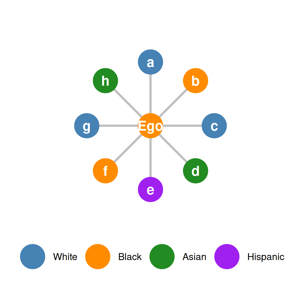
- Example: ego identifies as Black. Alters shaded the same color as ego share ego’s identity (“internal”); all others are “external.”
- \(E\) = number of “External” alters (different from you); \(I\) = number of “Internal” alters (same as you).
\[EI = \frac{E - I}{E + I}\]
Homophily: Worked Example and Interpretation
- Here: \(E = 6\), \(I = 2\) (alters b and f are Black, like ego).
\[EI = \frac{6 - 2}{6 + 2} = \frac{4}{8} = +0.5\]
- Negative EI: preference for “internal” ties. An EI of \(-1.0\) is maximum homophily.
- Positive EI: preference for “external” ties. An EI of \(+1.0\) is maximum heterophily.
- EI = 0: no preference — equal numbers of internal and external ties. Here, ego’s ties lean external.
Homophily: A Homophilous Example
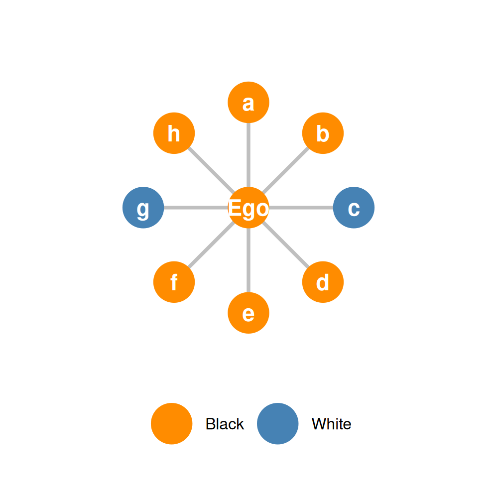
- Flip the pattern: ego (Black) now has 6 Black alters and 2 White alters (c and g).
\[EI = \frac{2 - 6}{2 + 6} = \frac{-4}{8} = -0.5\]
- Same magnitude as before, but on the homophily side: ego’s ties lean internal.
Diversity: Blau’s Index
- Tells us whether you tend to connect with a wide range of others on some sociodemographic characteristic.
- Given by Blau’s index of heterogeneity (\(H\)):
\[H = 1 - \sum_{k} p_k^2\]
Steps:
- Compute the proportion \(p_k\) of alters in each group \(k\).
- Square each proportion and sum them.
- Subtract from 1.0.
Diversity: Worked Example
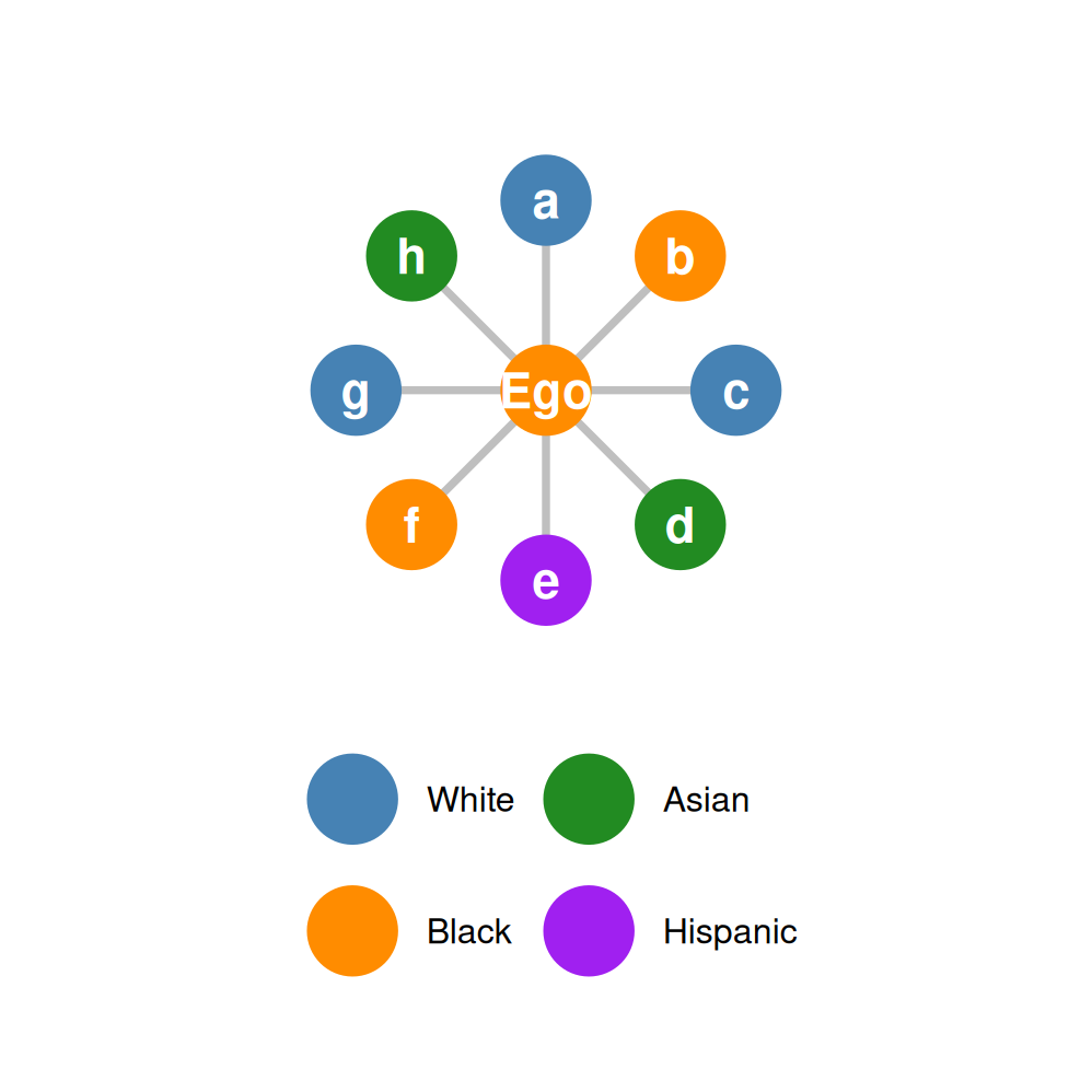
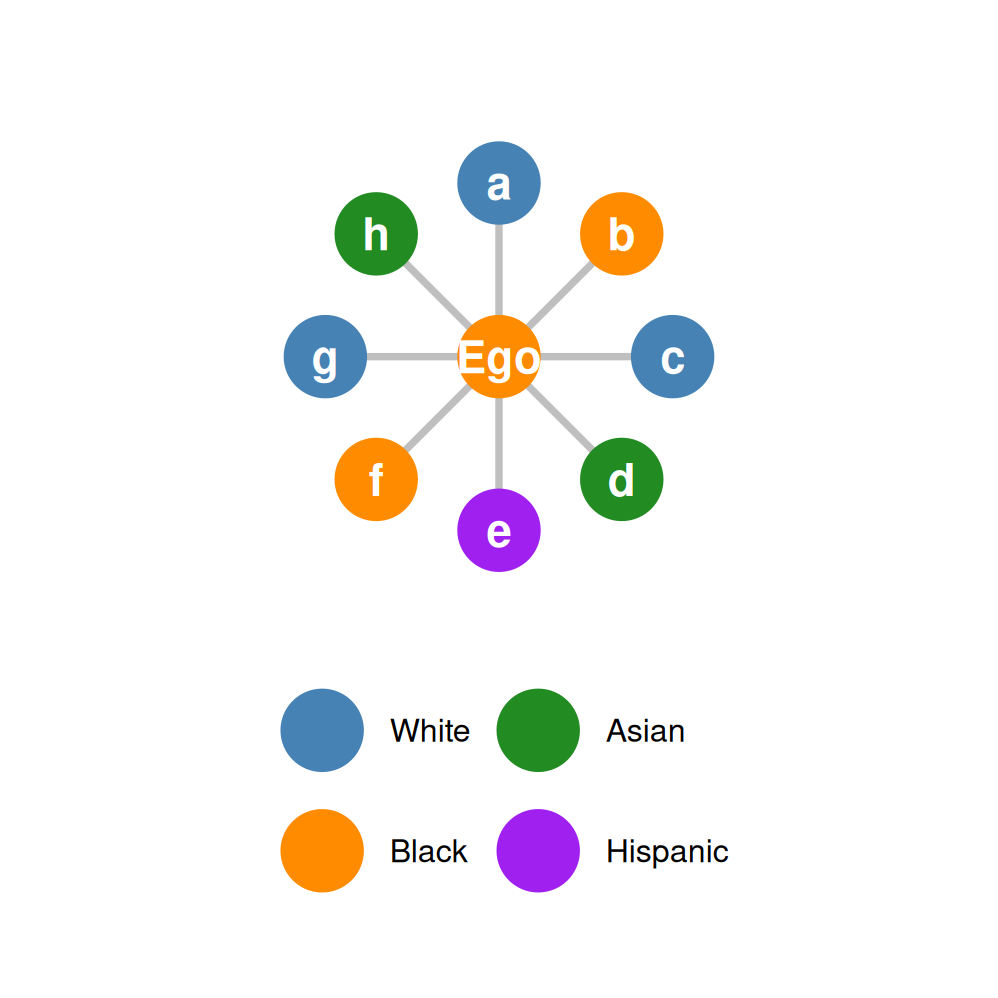
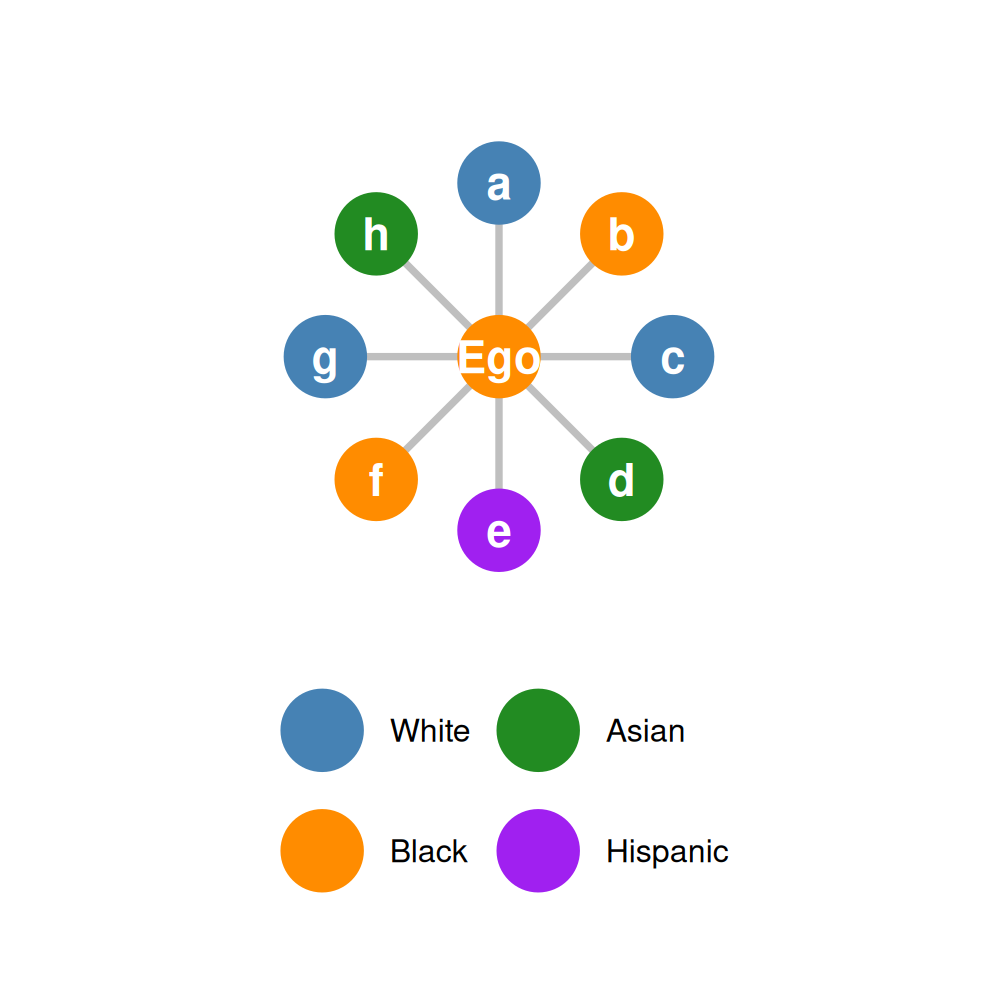
- Eight alters: 3 White, 2 Black, 2 Asian, 1 Hispanic.
- Step 1, proportions of alters in each group: \(p_{\text{W}} = \tfrac{3}{8} = 0.375\), \(p_{\text{B}} = \tfrac{2}{8} = 0.250\), \(p_{\text{A}} = \tfrac{2}{8} = 0.250\), \(p_{\text{H}} = \tfrac{1}{8} = 0.125\).
- Steps 2–3, square each proportion, sum, and subtract from 1.0:
\[H = 1 - \left(0.375^2 + 0.250^2 + 0.250^2 + 0.125^2\right)\]
\[= 1 - 0.281 = 0.72\]
Diversity: Interpreting \(H\)
- A completely homogeneous ego network has \(H = 0\) — no diversity among alters.
- The more diverse the ego network, the closer \(H\) is to 1.0.
- \(H\) is at a maximum (\(H_{max} = 1 - 1/k\)) when alters are spread evenly across \(k\) groups. With \(k = 4\): \(H_{max} = 0.75\), so \(H/H_{max} = 0.96\).
Diversity: A Low-Diversity Example
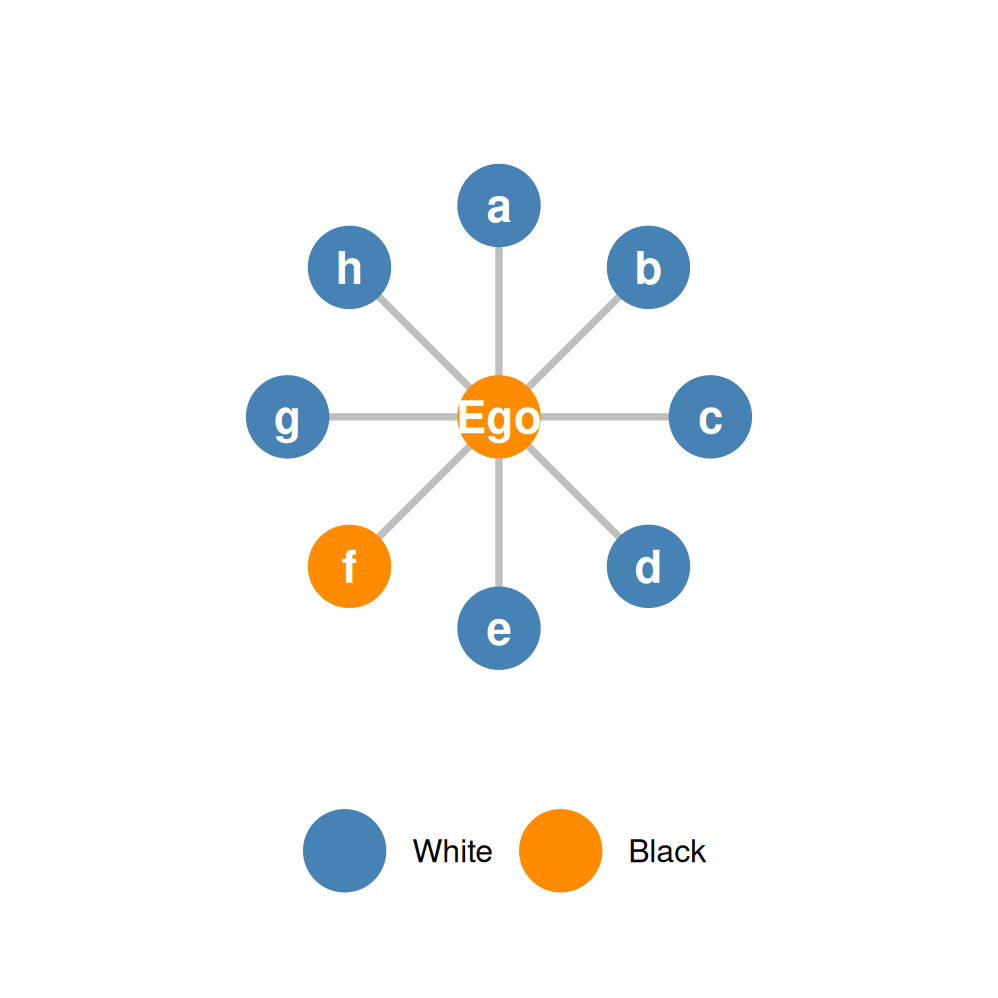
- Reverse the pattern: ego (Black) now has 7 White alters and 1 Black alter (f). Only \(k = 2\) groups are present.
Step 1: \(p_{\text{W}} = \tfrac{7}{8} = 0.875\), \(p_{\text{B}} = \tfrac{1}{8} = 0.125\).
Steps 2–3:
\[H = 1 - \left(0.875^2 + 0.125^2\right) = 1 - 0.781 = 0.22\]
- Far below the \(H = 0.72\) of the diverse network. With \(k = 2\): \(H_{max} = 0.5\), so \(H/H_{max} = 0.44\) — alters crowd into one group.
Clustering
- Tells us the extent to which your alters are interconnected among themselves (know one another) versus strangers to one another.
Given by the clustering coefficient (\(CC_i\)). You need:
- The number of alter-alter ties (\(m\))
- The number of alters (\(n\))
- Don’t care about the ego-alter links!
\[CC_i = \frac{2m}{n(n-1)}\]
Clustering: A Clustered Example
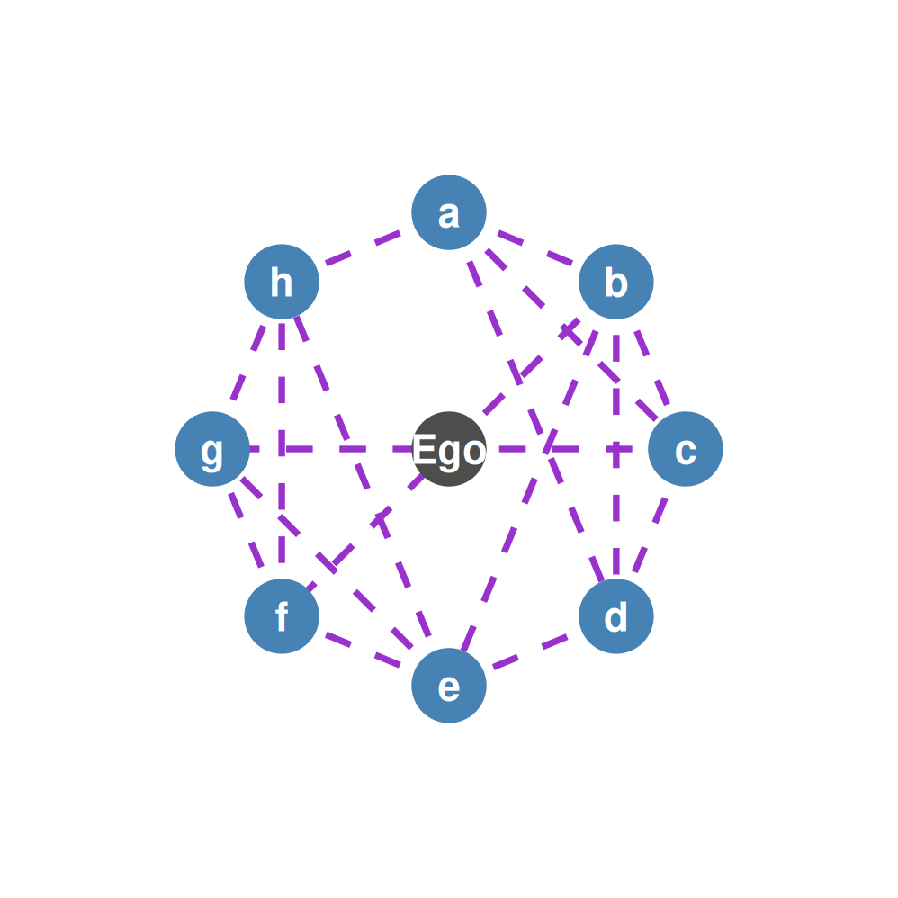
- \(n = 8\) alters; \(m = 17\) alter-alter ties.
\[CC_i = \frac{2 \times 17}{8 \times 7} = \frac{34}{56} = 0.61\]
- The ties are concentrated: two dense friend circles — everyone knows everyone within their circle — plus a handful of cross-circle ties.
- The clustering coefficient is the density of the network formed among your alters — the probability that two randomly chosen people you know also know one another.
Clustering: A Less Clustered Example
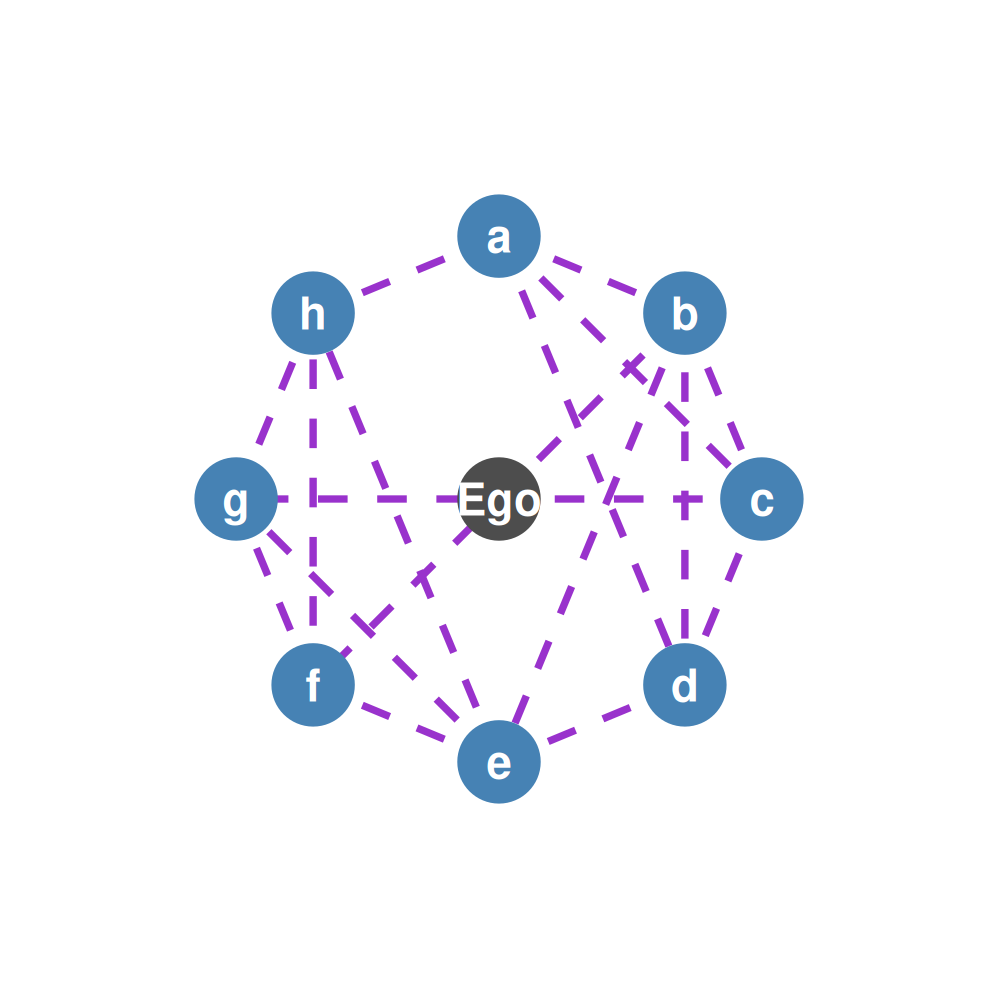
- Same number of alters (\(n = 8\)), but only \(m = 7\) alter-alter ties.
\[CC_i = \frac{2 \times 7}{8 \times 7} = \frac{14}{56} = 0.25\]
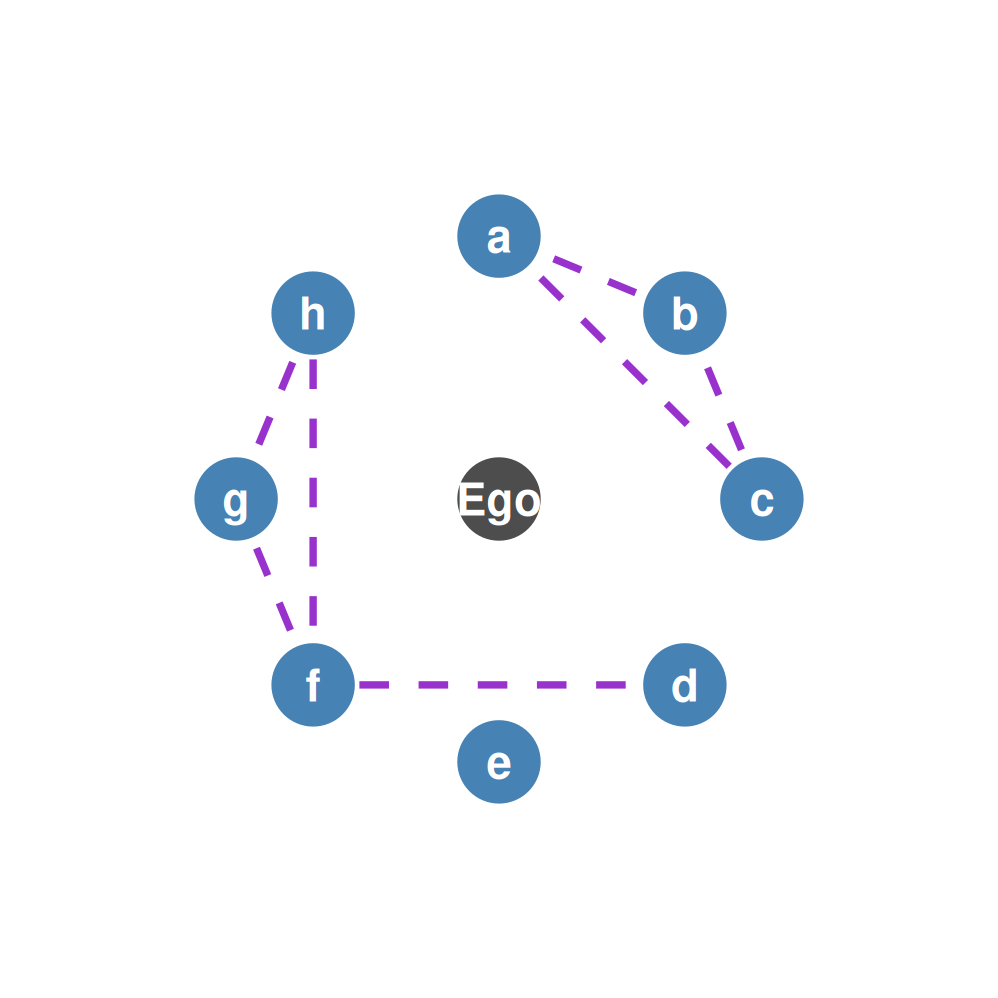
- The ties are thinner: two tight triangles of mutual friends, joined by a single bridge.
- Same-size ego networks can differ sharply in how concentrated their alter-alter ties are — and the clustering coefficient picks this up.
Clustering: The Extremes
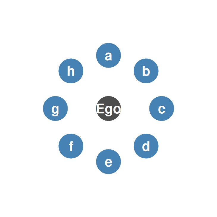
CC = 0.0 (\(m = 0\)): none of your friends know one another.
CC = 1.0 (\(m = 28\)): every one of your friends knows one another.