Directed Graph Metrics
The Basics of Social Network Analysis
Neighborhoods in Directed Graphs (1)
- Because links are directional, nodes have two neighborhoods.
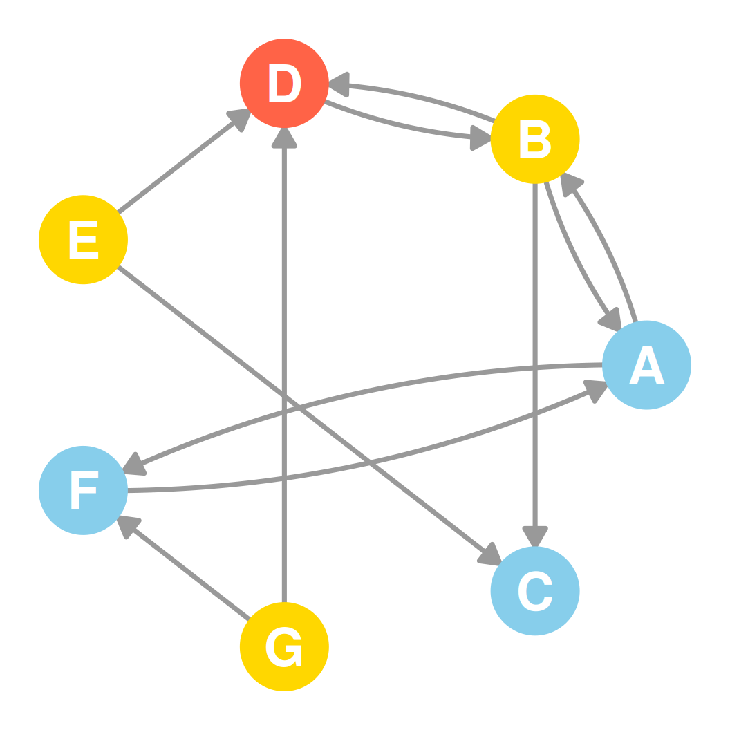
- In-Neighborhood (\(N^{in}(v)\)):
- Set of source nodes pointing to \(v\).
- Example: \(N^{in}(D) = \{B, E, G\}\) (highlighted in gold, pointing to focal node D in tomato).
Neighborhoods in Directed Graphs (2)
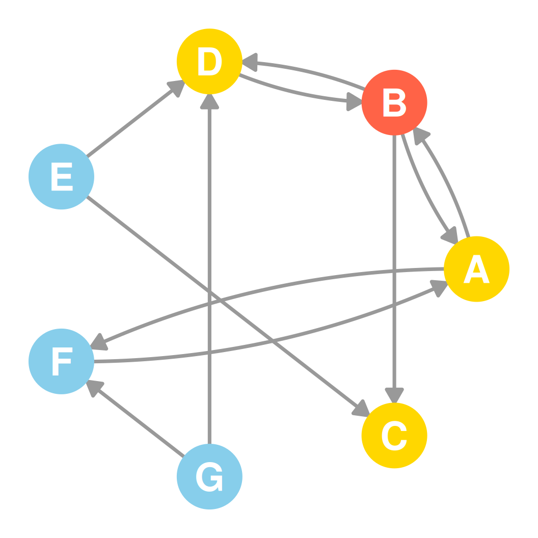
- Out-Neighborhood (\(N^{out}(v)\)):
- Set of destination nodes that \(v\) points to.
- Example: \(N^{out}(B) = \{A, C, D\}\) (highlighted in gold, pointing from focal node B in tomato).
Directed Neighborhoods: Reciprocity
- A node appears in both neighborhoods only if there is a reciprocal (mutual) tie.
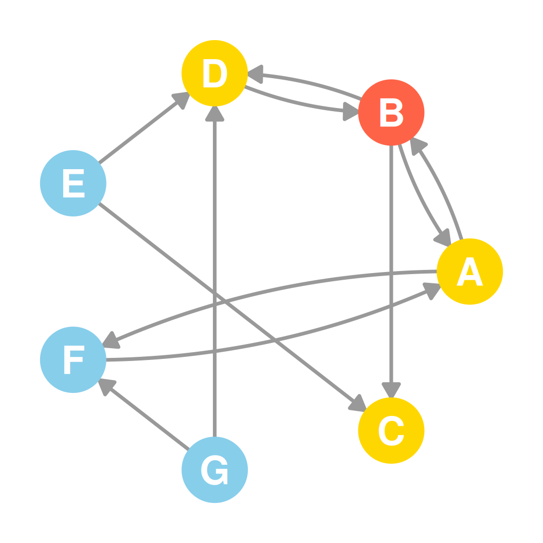
- Example for Node B (in tomato):
- In-Neighborhood: \(N^{in}(B) = \{A, D\}\)
- Out-Neighborhood: \(N^{out}(B) = \{A, C, D\}\)
Directed Neighborhoods: Reciprocity Overlap
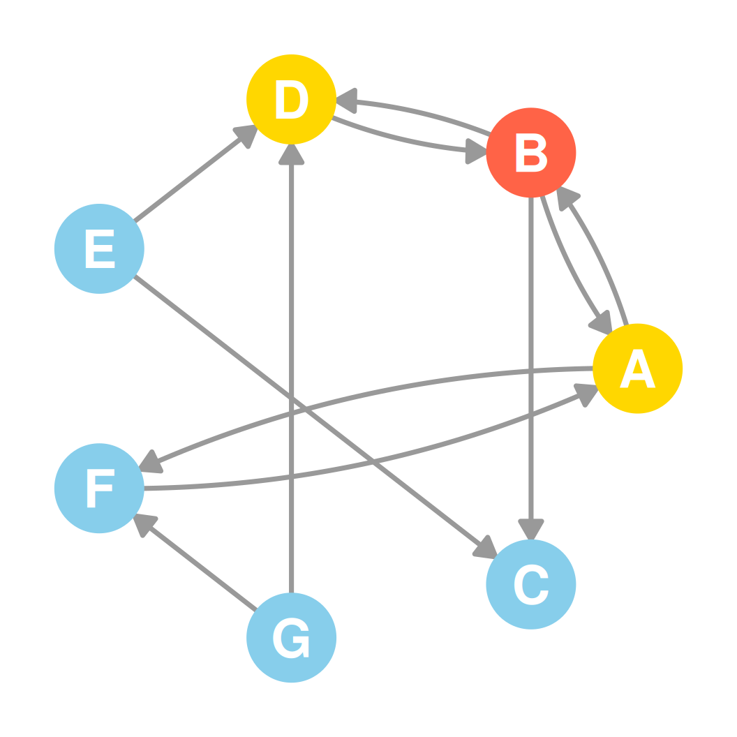
- Since there are reciprocal ties \(A \leftrightarrow B\) and \(B \leftrightarrow D\), nodes A and D (in gold) belong to both sets.
- Therefore, the overlap is the intersection of these two neighborhoods: \[N^{in}(B) \cap N^{out}(B) = \{A, D\}\]
Directed Neighborhood Intersection
- In directed graphs, neighborhood intersections can be defined for incoming or outgoing ties:
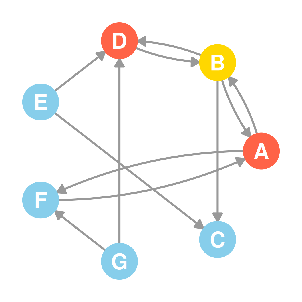
- In-Neighborhood Intersection: Common source nodes pointing to both \(u\) and \(v\):
- \(N^{in}(D) \cap N^{in}(A) = \{B\}\) (focal nodes \(D\) and \(A\) in tomato; common source \(B\) in gold)
- Out-Neighborhood Intersection: Common destination nodes that both \(u\) and \(v\) point to:
- \(N^{out}(B) \cap N^{out}(E) = \{C, D\}\) (shown on the next slide)
Directed Neighborhood Intersection: Example
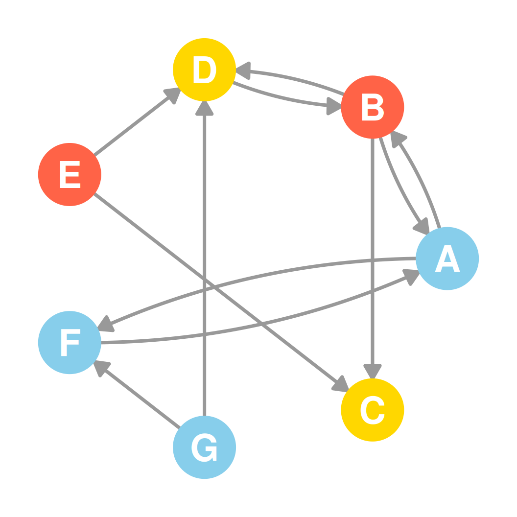
- Let’s visualize the out-neighborhood intersection of nodes B and E (in tomato):
- \(N^{out}(B) = \{A, C, D\}\)
- \(N^{out}(E) = \{C, D\}\)
- They share two common destination nodes:
- \(N^{out}(B) \cap N^{out}(E) = \{C, D\}\) (in gold)
Directed Neighborhood Union
- Similarly, directed neighborhood unions combine the sets of neighbors:
- In-Neighborhood Union: Nodes pointing to either \(u\) or \(v\):
- \(N^{in}(D) \cup N^{in}(A) = \{B, E, F, G\}\) (focal nodes \(D\) and \(A\) in tomato; union members in gold)
- Out-Neighborhood Union: Nodes that either \(u\) or \(v\) points to:
- \(N^{out}(B) \cup N^{out}(E) = \{A, C, D\}\) (shown on the next slide)
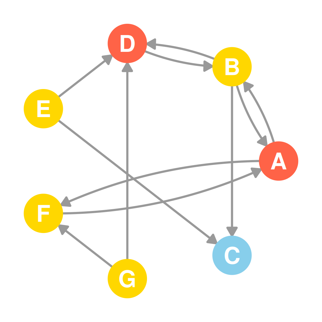
Directed Neighborhood Union: Example
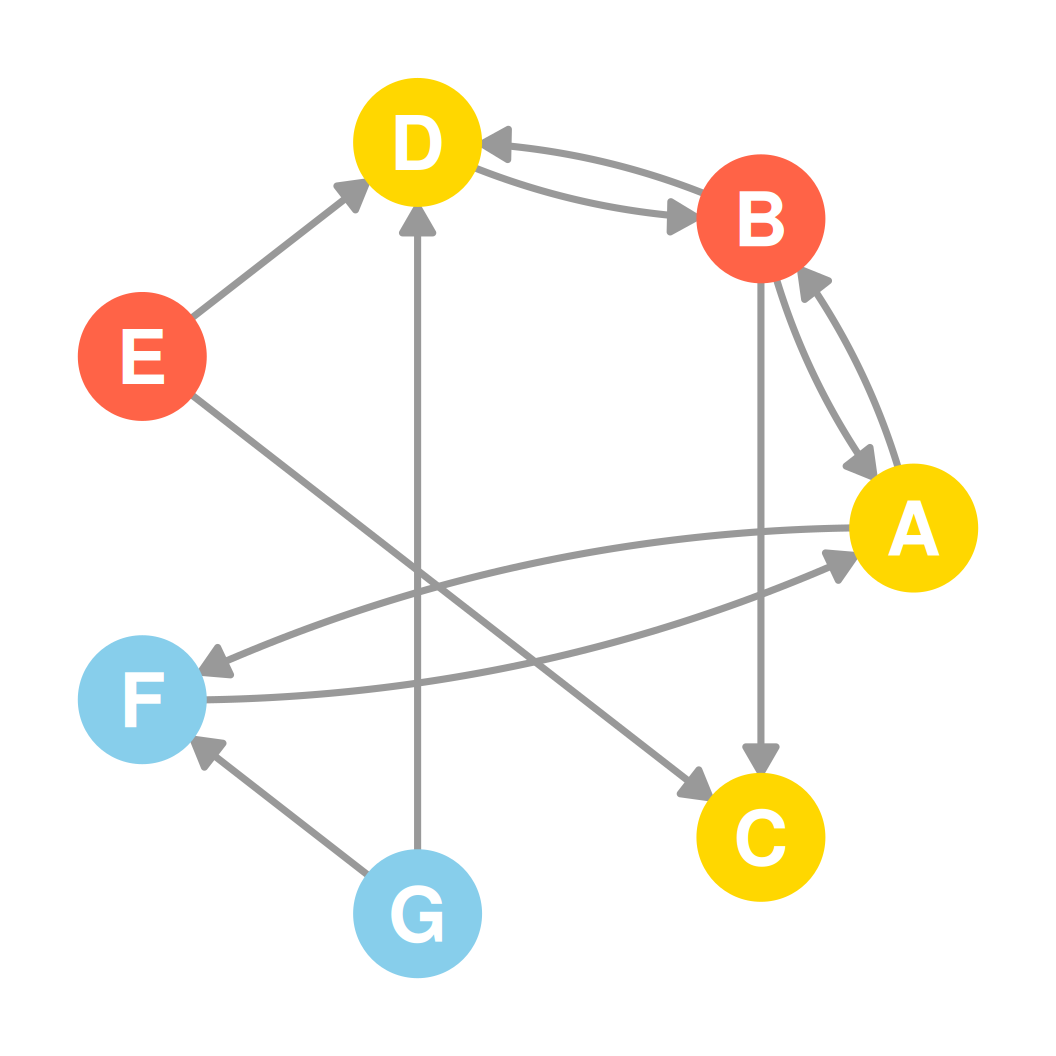
- Let’s visualize the out-neighborhood union of nodes B and E (in tomato):
- \(N^{out}(B) = \{A, C, D\}\)
- \(N^{out}(E) = \{C, D\}\)
- Combining all unique destination nodes gives:
- \(N^{out}(B) \cup N^{out}(E) = \{A, C, D\}\) (in gold)
Indegree: An Example
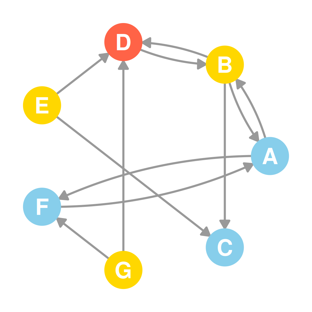
- Let’s find the indegree for Node D (in tomato) on the right:
- Source nodes pointing to D: \(N^{in}(D) = \{B, E, G\}\) (in gold)
- Indegree: \(k^{in}_D = |N^{in}(D)| = 3\)
- Node D has 3 incoming arrows, representing a node with relatively high popularity or status.
Outdegree: An Example
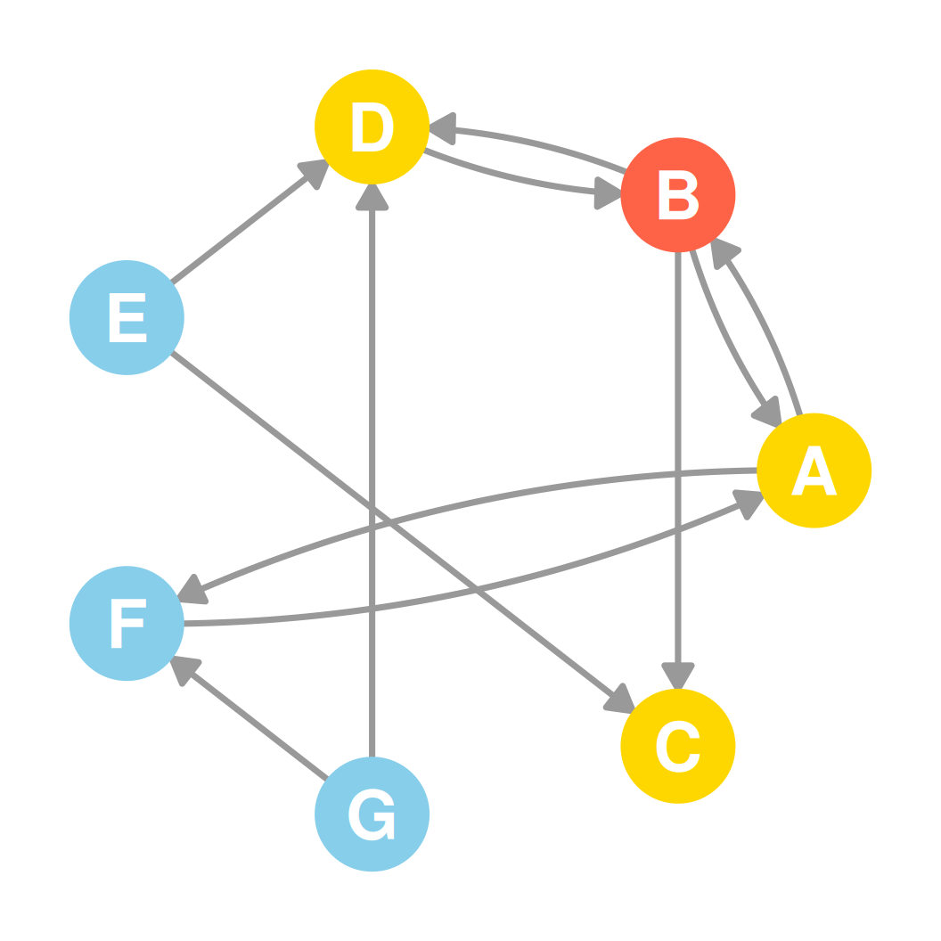
- Let’s find the outdegree for Node B (in tomato) on the right:
- Target nodes that B points to: \(N^{out}(B) = \{A, C, D\}\) (in gold)
- Outdegree: \(k^{out}_B = |N^{out}(B)| = 3\)
- Node B has 3 outgoing arrows, representing a node with relatively high sociability or activity.
Node Types: An Example
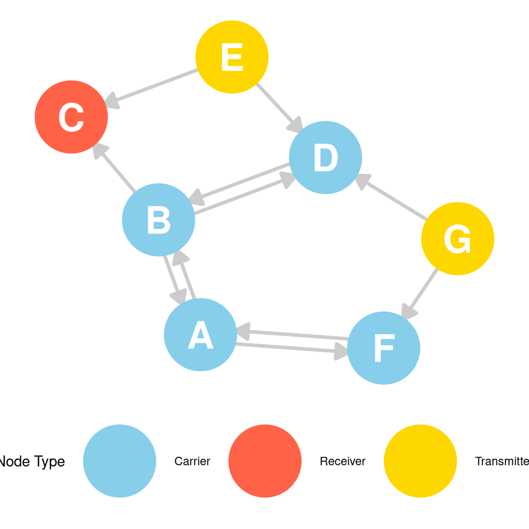
- Looking at the directed graph on the right:
- Receiver: Node C (only receives ties).
- Transmitters: Nodes E and G (only send ties).
- Carriers: Nodes A, B, D, F (both receive and send ties).
Directed Degree Sets & Sequences
- Directed graphs have two distinct degree sets and two distinct degree sequences—one of each for in-degree and out-degree.
- For our 7-node directed graph (shown on the right):
- In-Degree Set: \(\{2, 2, 2, 3, 0, 2, 0\}\)
- In-Degree Sequence: \((3, 2, 2, 2, 2, 0, 0)\)
- Out-Degree Set: \(\{2, 3, 0, 1, 2, 1, 2\}\)
- Out-Degree Sequence: \((3, 2, 2, 2, 1, 1, 0)\)
Directed Range & Sum: Example (In-Degree)
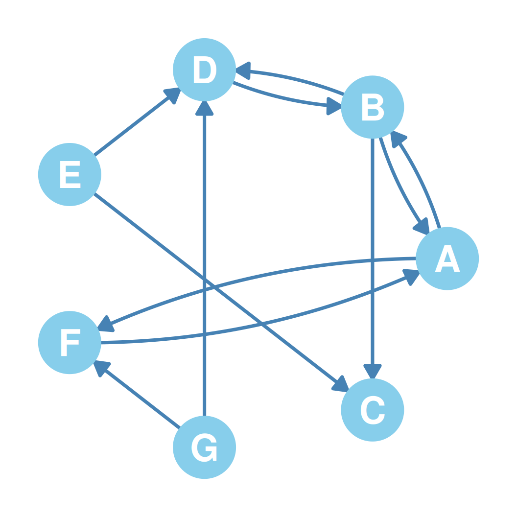
- For our 7-node directed graph (shown again on the right, \(m = 11\)):
- In-Degrees: \(k^{in} = (2, 2, 2, 3, 0, 2, 0)\)
- \(k^{in}_{max} = 3\) (Node D), \(k^{in}_{min} = 0\) (Nodes E and G)
- Range \(k^{in}_r = 3 - 0 = 3\)
- Sum \(\sum k^{in}_i = 2+2+2+3+0+2+0 = 11\)
- In-Degrees: \(k^{in} = (2, 2, 2, 3, 0, 2, 0)\)
Directed Range & Sum: Example (Out-Degree)
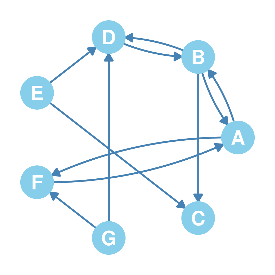
- For our 7-node directed graph (shown again on the right, \(m = 11\)):
- Out-Degrees: \(k^{out} = (2, 3, 0, 1, 2, 1, 2)\)
- \(k^{out}_{max} = 3\) (Node B), \(k^{out}_{min} = 0\) (Node C)
- Range \(k^{out}_r = 3 - 0 = 3\)
- Sum \(\sum k^{out}_i = 2+3+0+1+2+1+2 = 11\)
- Out-Degrees: \(k^{out} = (2, 3, 0, 1, 2, 1, 2)\)
Order and Size: Directed Example
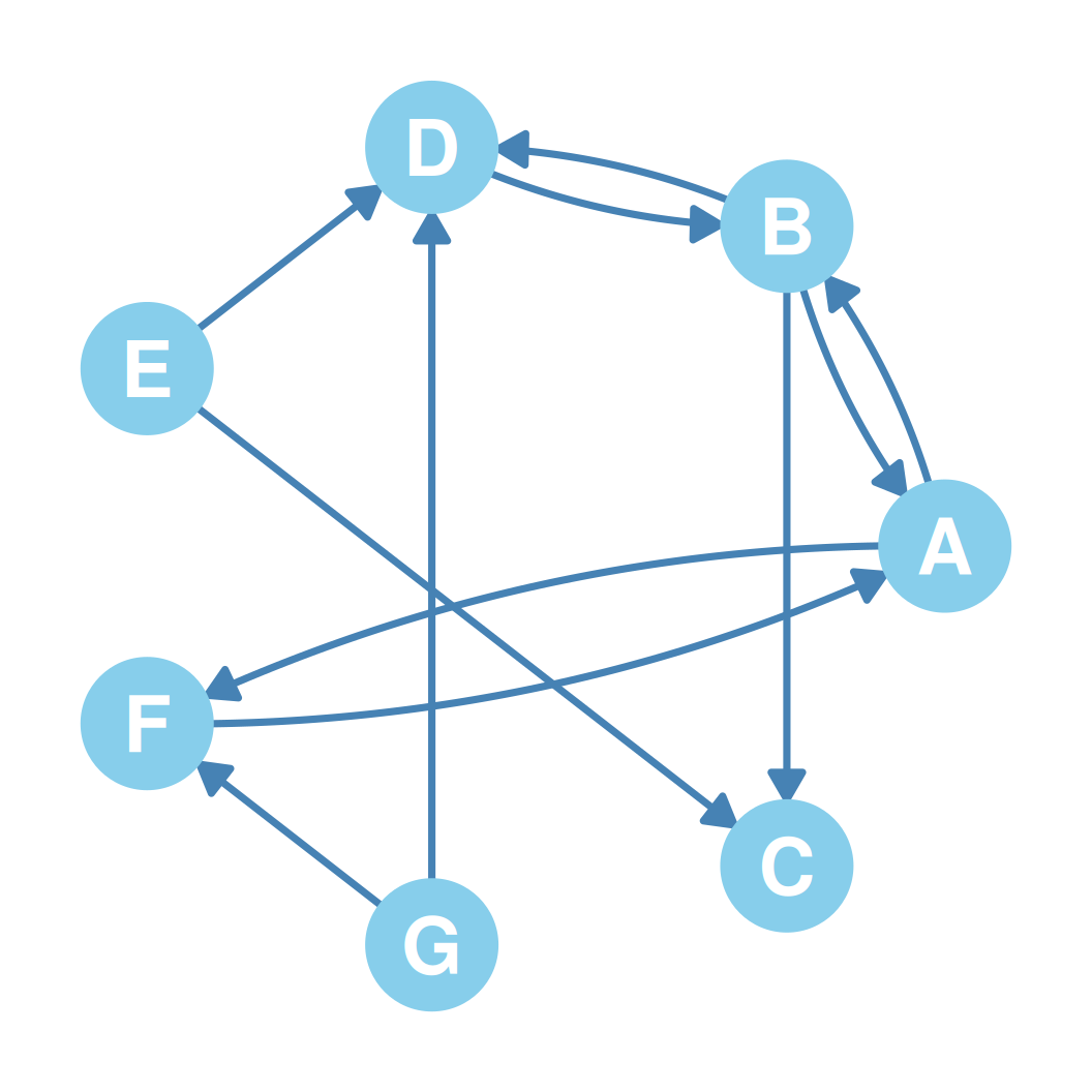
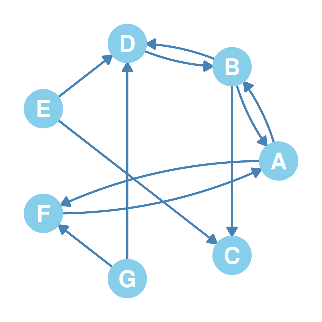
- Let’s look at the directed graph on the right:
- Node Set (\(V\)): \(\{A, B, C, D, E, F, G\}\)
- Edge Set (\(E\)): \(\{AB, AF, BA, BD,\)
\(BC, DB, EC, ED,\)
\(FA, GF, GD\}\) - Graph Order (\(n = |V|\)): 7 nodes
- Graph Size (\(m = |E|\)): 11 edges
- In directed graphs, edges are ordered pairs:
- The order in which the nodes are listed matters: \(AB\) (from \(A\) to \(B\)) is a different edge than \(BA\) (from \(B\) to \(A\)).
- That’s why both \(AB\) and \(BA\) can appear in the edge set above.
Maximum Size: Directed Example
- Let’s look at the directed graph on the right:
- Order (\(n\)): 7 nodes
- Formula: \[Max(E) = n(n - 1)\]
Maximum Size: Directed Calculation
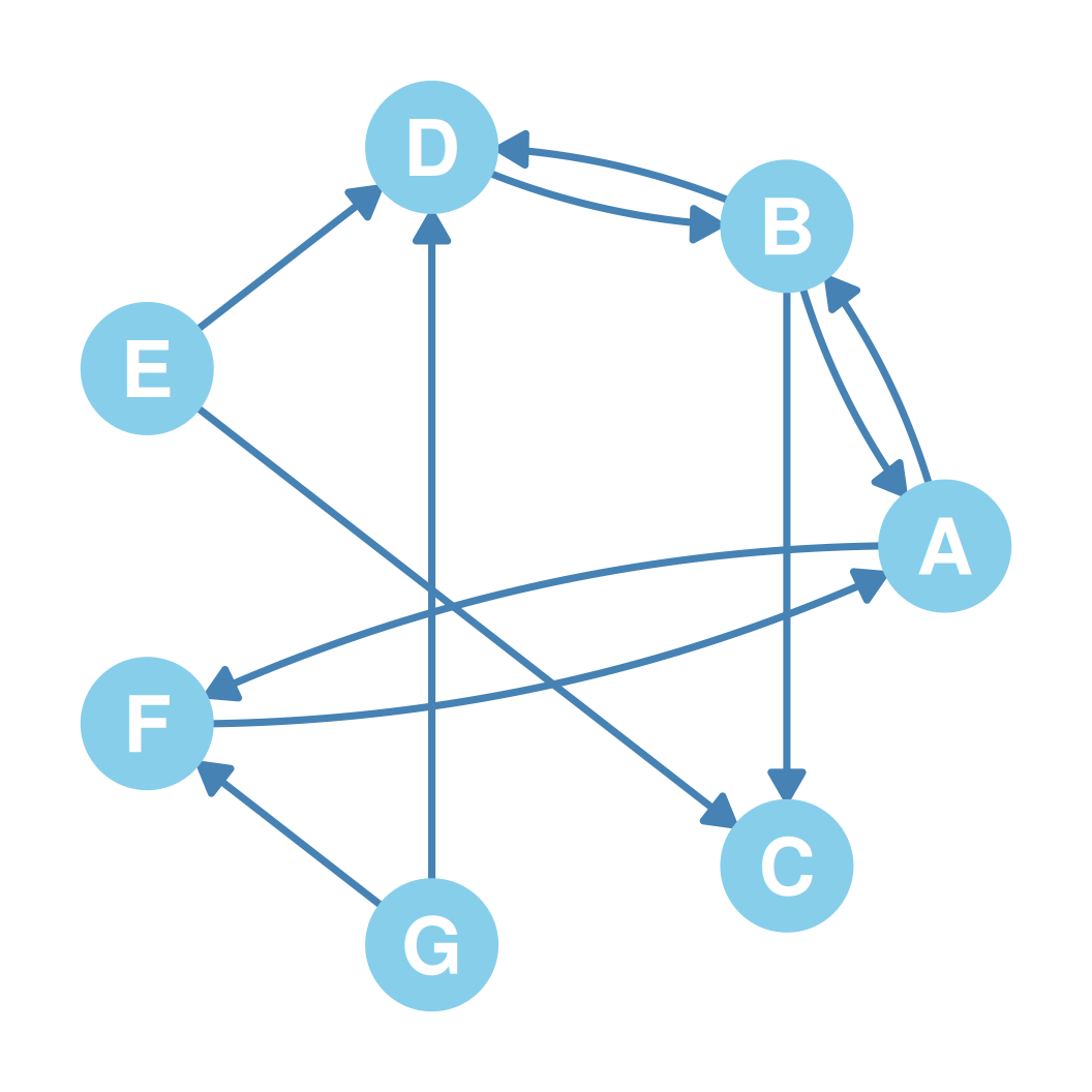
- Order (\(n\)): 7 nodes (shown on the right)
- Maximum possible size calculation: \[Max(E) = 7 \times (7 - 1) = 7 \times 6 = 42\text{ edges}\]
- Interpretation:
- A complete directed graph with 7 nodes would have exactly 42 directed arcs.
Density: Directed Example
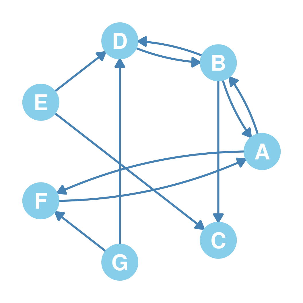
- Let’s look at the directed graph on the right:
- Order (\(n\)): 7 nodes
- Size (\(m\)): 11 directed edges
- Maximum possible edges: \[Max(E) = 7 \times 6 = 42\]
Density: Directed Calculation
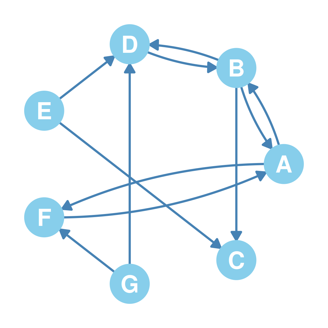
- Observed directed edges (\(m\)): 11 (shown on the right)
- Maximum possible edges: 42
- Density Formula: \[d = \frac{m}{Max(E)} = \frac{11}{42} \approx 0.262\]
- Interpretation:
- Exactly 26.2% of all possible directed ties are present in this network.
Equivalence of Means: Example
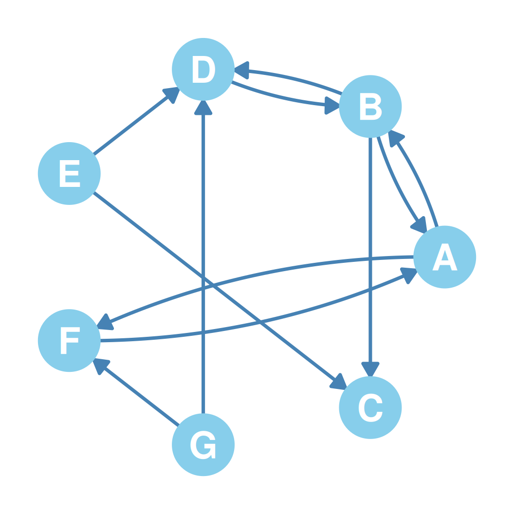
- In our 7-node directed graph:
- Order (\(n\)): 7 nodes
- Size (\(m\)): 11 directed edges
- Mean In-Degree: \(\bar{k}^{in} = \frac{2+2+2+3+0+2+0}{7} = \frac{11}{7} \approx 1.57\)
- Mean Out-Degree: \(\bar{k}^{out} = \frac{2+3+0+1+2+1+2}{7} = \frac{11}{7} \approx 1.57\)
- They are equal! (\(\bar{k}^{in} = \bar{k}^{out} = 1.57 = m/n\))
Directed Degree Variance: Example (In-Degree)
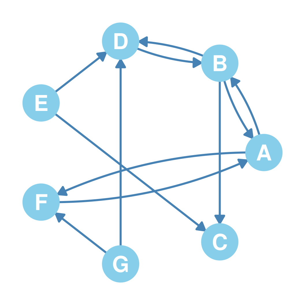
- In our 7-node directed graph:
- Mean degree (\(\bar{k}\)) is \(\approx 1.57\)
- In-Degree Variance (\(\sigma^2_{in}\)):
- Values:
- \(k^{in} = (2, 2, 2, 3, 0, 2, 0)\)
- Calculation:
- \(\frac{4 \times (2-1.57)^2 + 1 \times (3-1.57)^2 + 2 \times (0-1.57)^2}{7} =\)
- \(\frac{4 \times 0.18 + 2.04 + 2 \times 2.47}{7} \approx 1.102\)
- Values:
Directed Degree Variance: Example (Out-Degree)
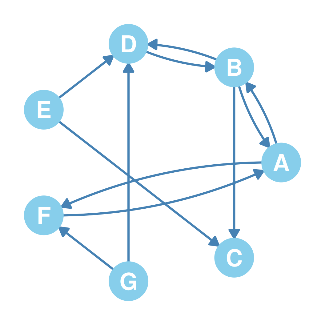
- In our 7-node directed graph:
- Mean degree (\(\bar{k}\)) is \(\approx 1.57\)
- Out-Degree Variance (\(\sigma^2_{out}\)):
- Values:
- \(k^{out} = (2, 3, 0, 1, 2, 1, 2)\)
- Calculation:
- \(\frac{3(2-1.57)^2 + (3-1.57)^2 + (0-1.57)^2 + 2(1-1.57)^2}{7} \approx 0.816\)
- Values:
- In-degree is more heterogeneous than out-degree in this network!
Symmetric Directed Graphs
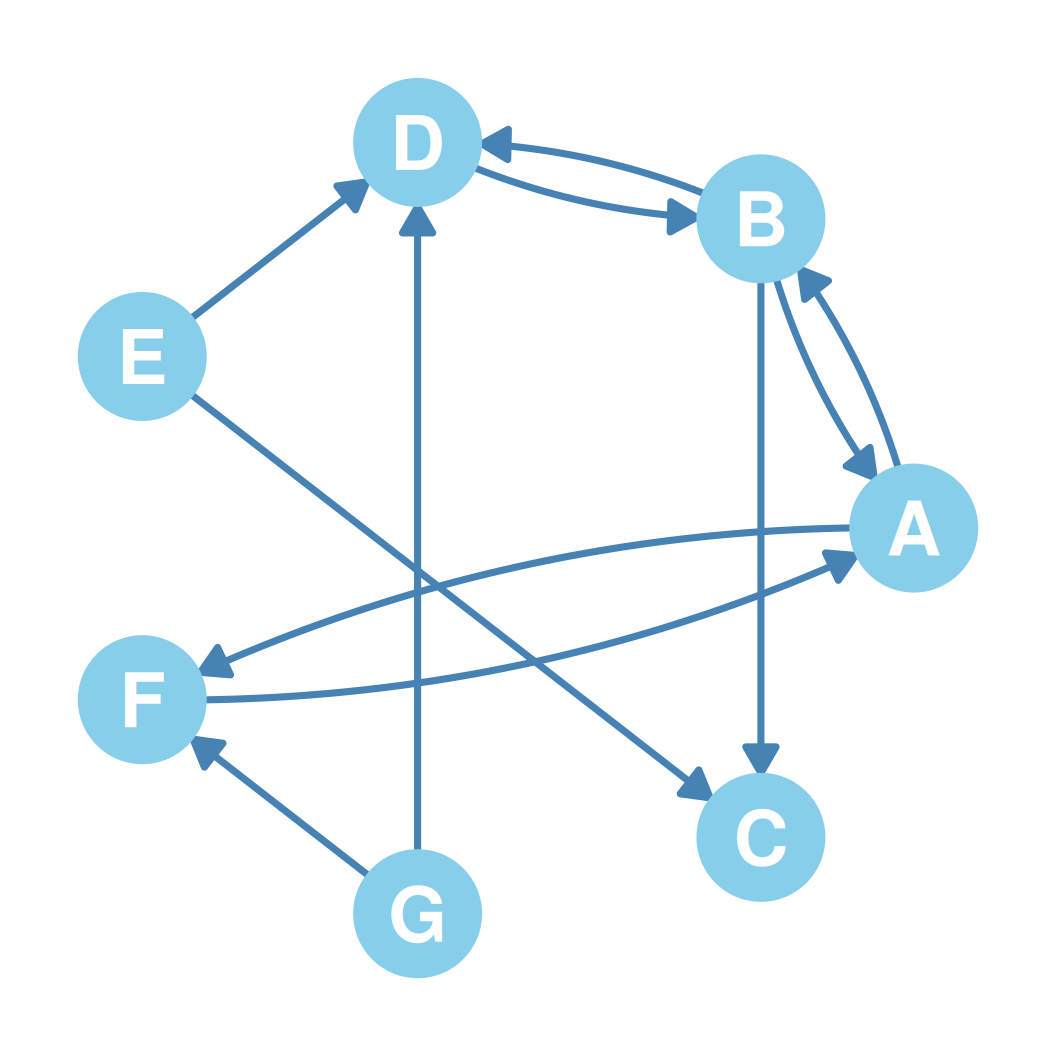
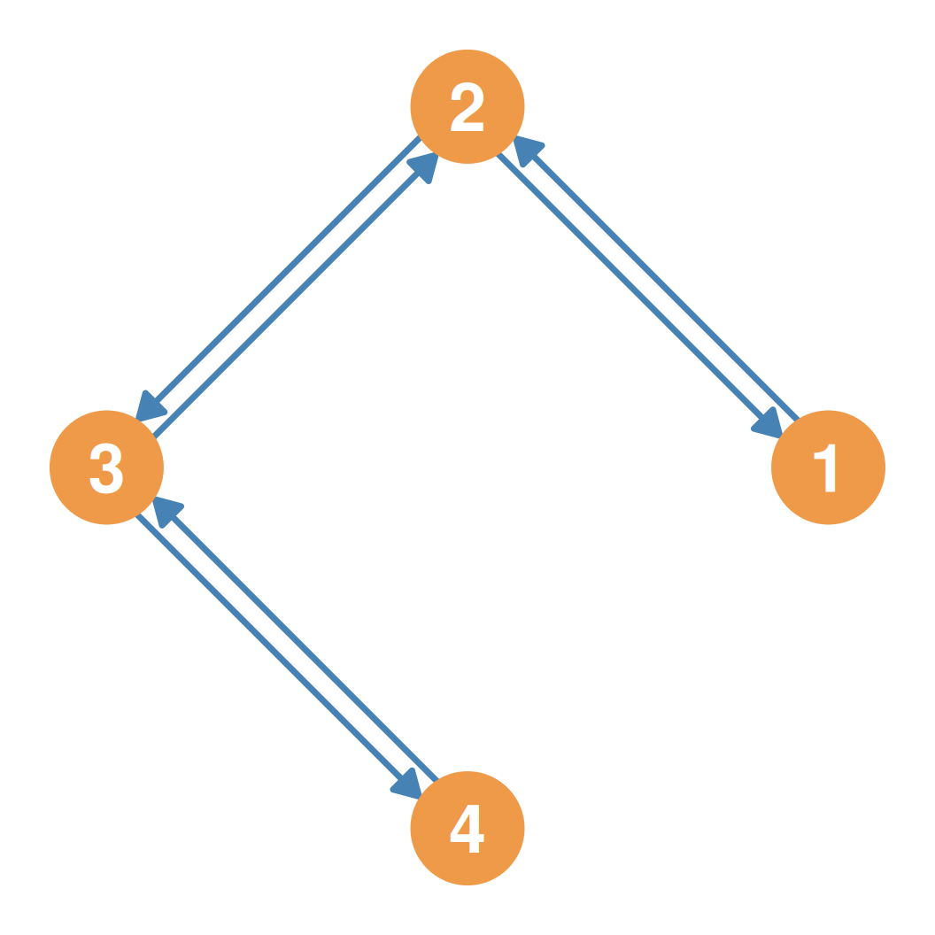
- Symmetric Directed Graph:
- A digraph where for every directed arc \(u \rightarrow v\), the reverse arc \(v \rightarrow u\) is also present.
- Formally: \(AB \iff BA\).
- Key Properties:
- It is a directed representation of an undirected (symmetric) graph.
- Every connected dyad is reciprocal (Mutual).
Functional Graphs
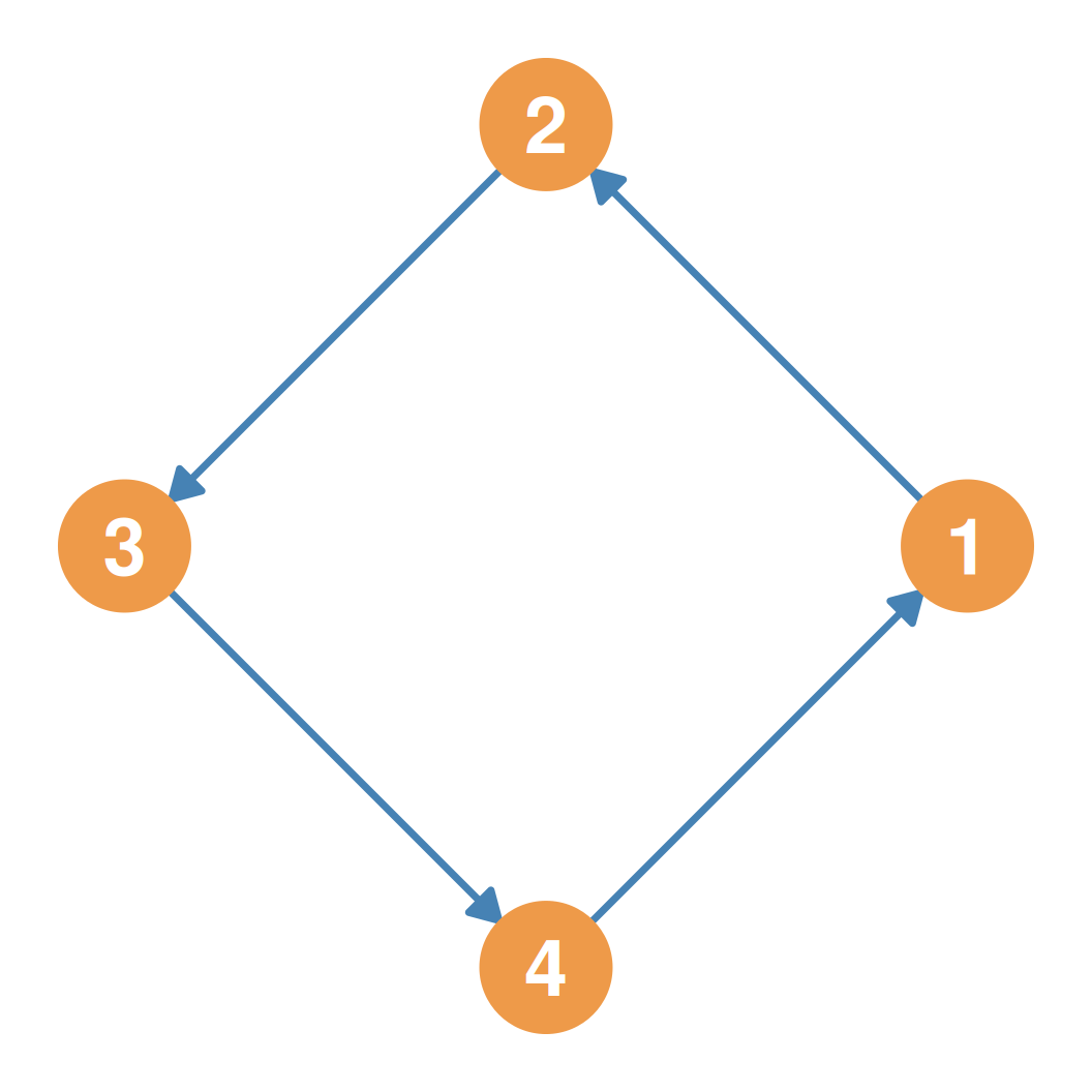
- Functional Graph:
- A directed graph where every node has an outdegree of exactly 1: \[k^{out}_v = 1 \quad \text{for all } v \in V\]
- Key Properties:
- Represents a single-valued function \(f: V \rightarrow V\), mapping each node to exactly one target.
- e.g., “Who is your best friend?” or “Who is your immediate boss?”
Oriented Graphs
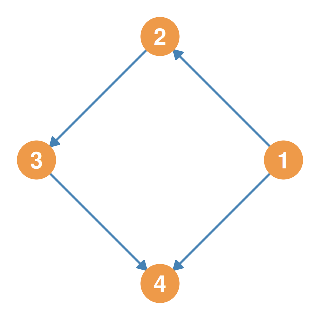
- Oriented Graph:
- A directed graph obtained by choosing a single direction for each edge in an undirected graph.
- Key Properties:
- No reciprocal (mutual) arcs can exist: if \(u \rightarrow v\) is present, then \(v \rightarrow u\) is forbidden.
- Represents purely non-reciprocal systems of interaction or asymmetric flows.
Directed Tree Graphs
- Directed Tree Graph:
- A directed, acyclic graph where a single root node has an indegree of 0, and all other nodes have an indegree of exactly 1: \[k^{in}_{root} = 0 \quad \text{and} \quad k^{in}_v = 1 \quad \text{for all other } v\]
- Key Properties:
- Naturally models strict authority hierarchies or family trees.
- Every node has exactly one parent or supervisor, with zero loops or overlapping chains of command.