Undirected Graph Metrics
The Basics of Social Network Analysis
Neighborhood Intersection
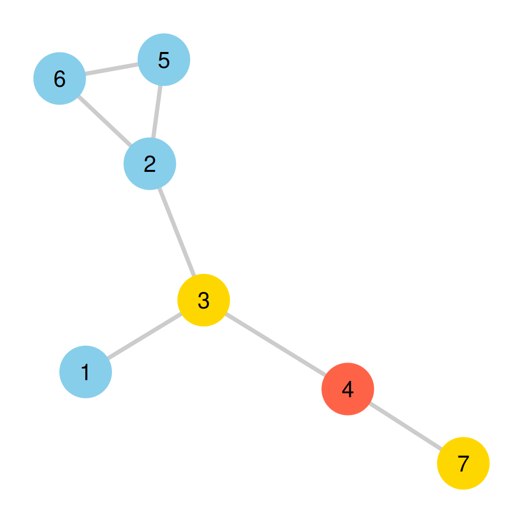
- Neighborhood Intersection (\(\mathcal{N}(u) \cap \mathcal{N}(v)\)) is the set of common neighbors connected to both \(u\) and \(v\).
- In our graph:
- \(N(1) = \{3\}\)
- \(N(4) = \{3, 7\}\)
- The intersection is the single node they share:
- \(N(1) \cap N(4) = \{3\}\)
Neighborhood Intersection: Example 2
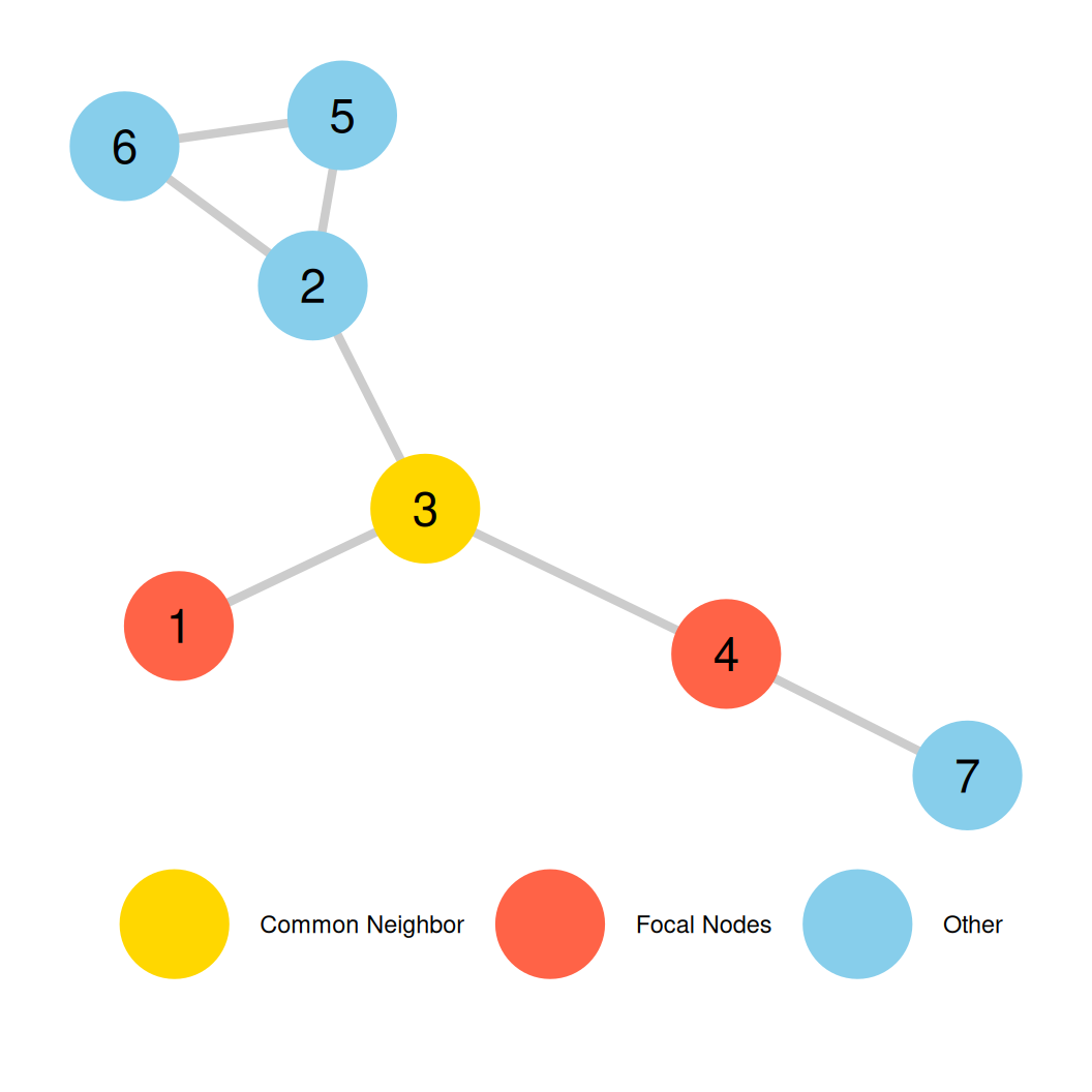
- Let’s find the neighborhood intersection of nodes 5 and 3.
- First, list their individual neighborhood sets:
- \(\mathcal{N}(5) = \{2, 6\}\)
- \(\mathcal{N}(3) = \{1, 2, 4\}\)
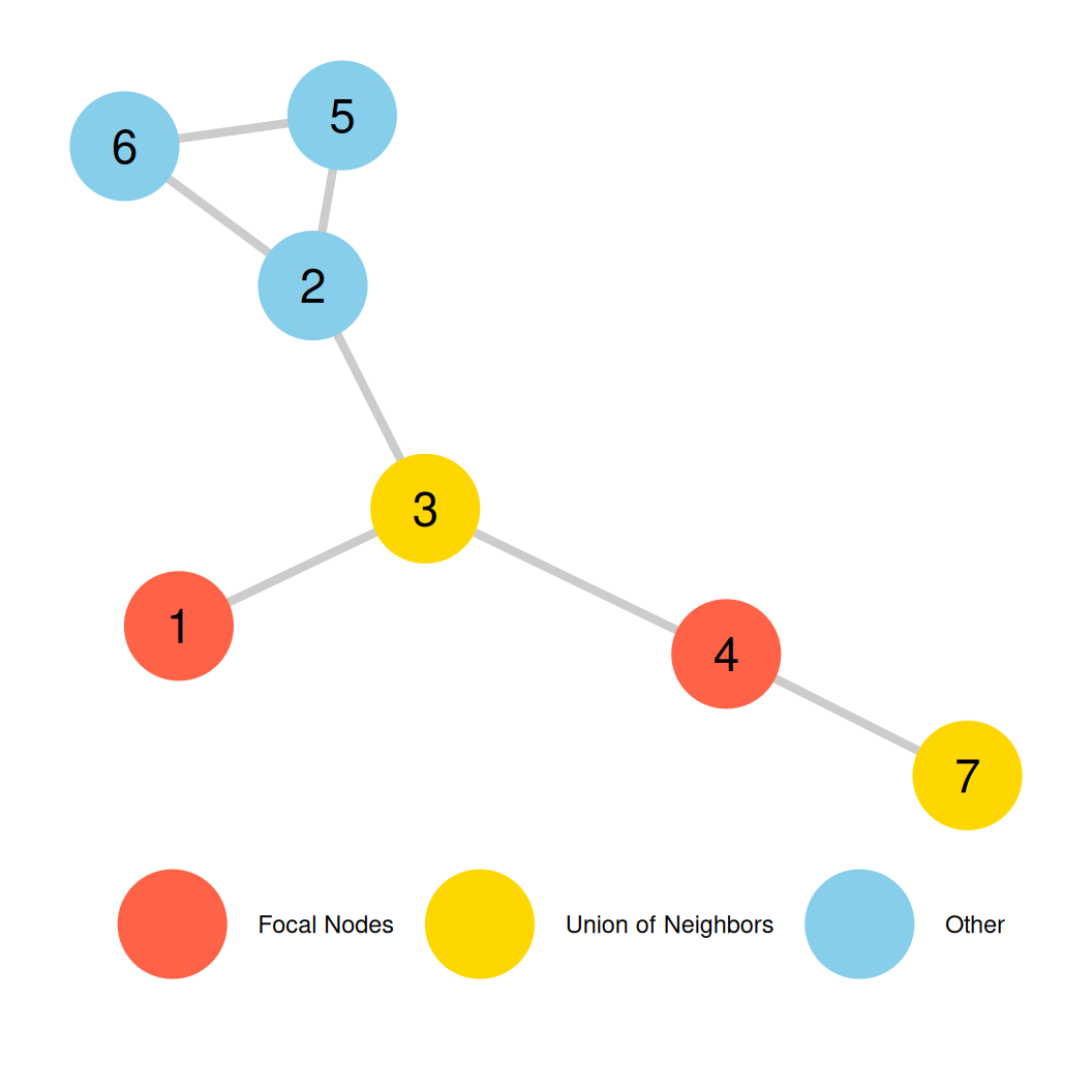
- Nodes 5 and 3 (in tomato) are not directly connected, but they share a common neighbor: node 2 (in gold).
- Therefore, their neighborhood intersection is: \[\mathcal{N}(5) \cap \mathcal{N}(3) = \{2\}\]
Neighborhood Union
- Neighborhood Union (\(\mathcal{N}(u) \cup \mathcal{N}(v)\)) is the set of all nodes connected to either \(u\) or \(v\).
- In our graph:
- \(N(1) = \{3\}\)
- \(N(4) = \{3, 7\}\)
- The union contains all unique neighbors from both sets:
- \(N(1) \cup N(4) = \{3, 7\}\)
Neighborhood Union: Example 2
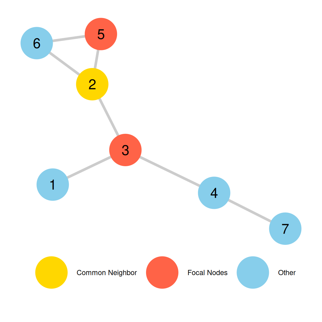
- Let’s find the neighborhood union of nodes 5 and 3.
- First, list their individual neighborhood sets:
- \(\mathcal{N}(5) = \{2, 6\}\)
- \(\mathcal{N}(3) = \{1, 2, 4\}\)
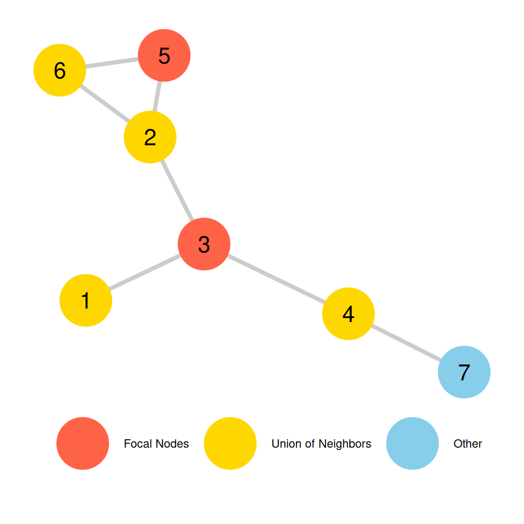
- Focal nodes 5 and 3 are shown in tomato; the union of their neighbors (nodes 1, 2, 4, 6) is shown in gold.
- Therefore, the union of neighbors is: \[\mathcal{N}(5) \cup \mathcal{N}(3) = \{1, 2, 4, 6\}\]
Node Degree: An Example
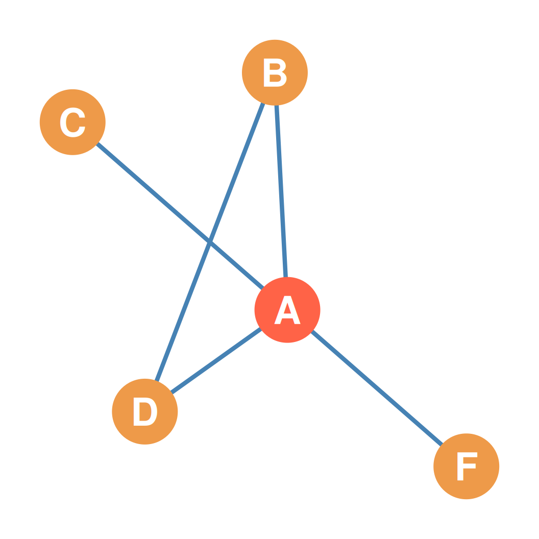
- Let’s calculate the degree for Node A (in tomato) on the right:
- Neighbors of A: \(\mathcal{N}(A) = \{B, C, D, F\}\)
- Neighborhood size: \(k_A = |\mathcal{N}(A)| = 4\)
- Incident edges: \(AB\), \(AC\), \(AD\), and \(AF\) (\(k_A = 4\))
- Thus, the degree of Node A is 4.
Endpoints: An Example
- Let’s identify the endpoints in the graph on the right:
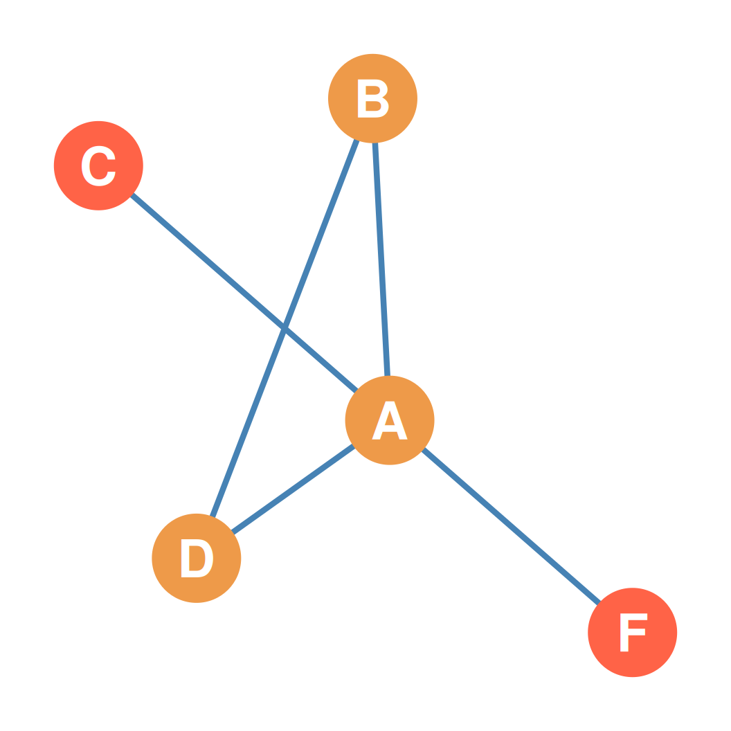
- Nodes C and F (in tomato) are connected only to node A.
- Since \(k_C = 1\) and \(k_F = 1\), they have degree one.
- Therefore, C and F are the endpoints of this graph.
Order and Size: Undirected Example
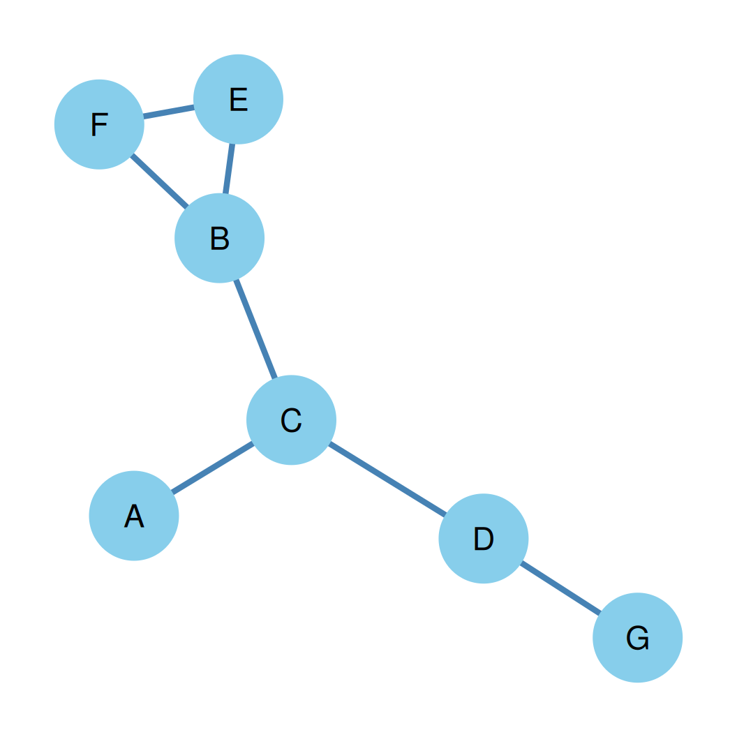
- Let’s look at the undirected graph on the right:
- Node Set (\(V\)): \(\{A, B, C, D, E, F, G\}\)
- Edge Set (\(E\)): \(\{AC, CD, DG,\)
\(BE, EF, FB, CB\}\) - Graph Order (\(n = |V|\)): 7 nodes
- Graph Size (\(m = |E|\)): 7 edges
Maximum Size: Undirected Example
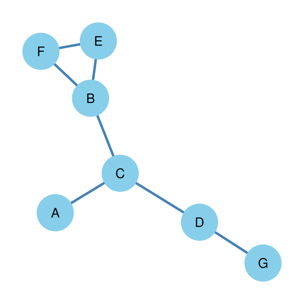
- Let’s look at the undirected graph on the right:
- Order (\(n\)): 7 nodes
- Formula: \[Max(E) = \frac{n(n - 1)}{2}\]
Maximum Size: Undirected Calculation
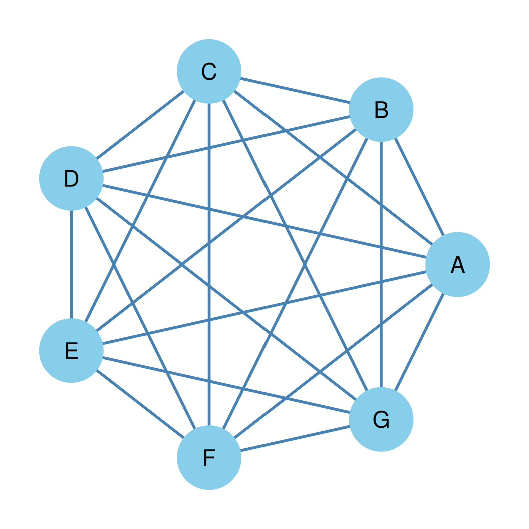
- Order (\(n\)): 7 nodes (shown on the right)
- Maximum possible size calculation: \[Max(E) = \frac{7 \times (7 - 1)}{2} = \frac{42}{2} = 21\text{ edges}\]
- Interpretation:
- A complete undirected graph with 7 nodes would have exactly 21 edges.
Density: Undirected Example
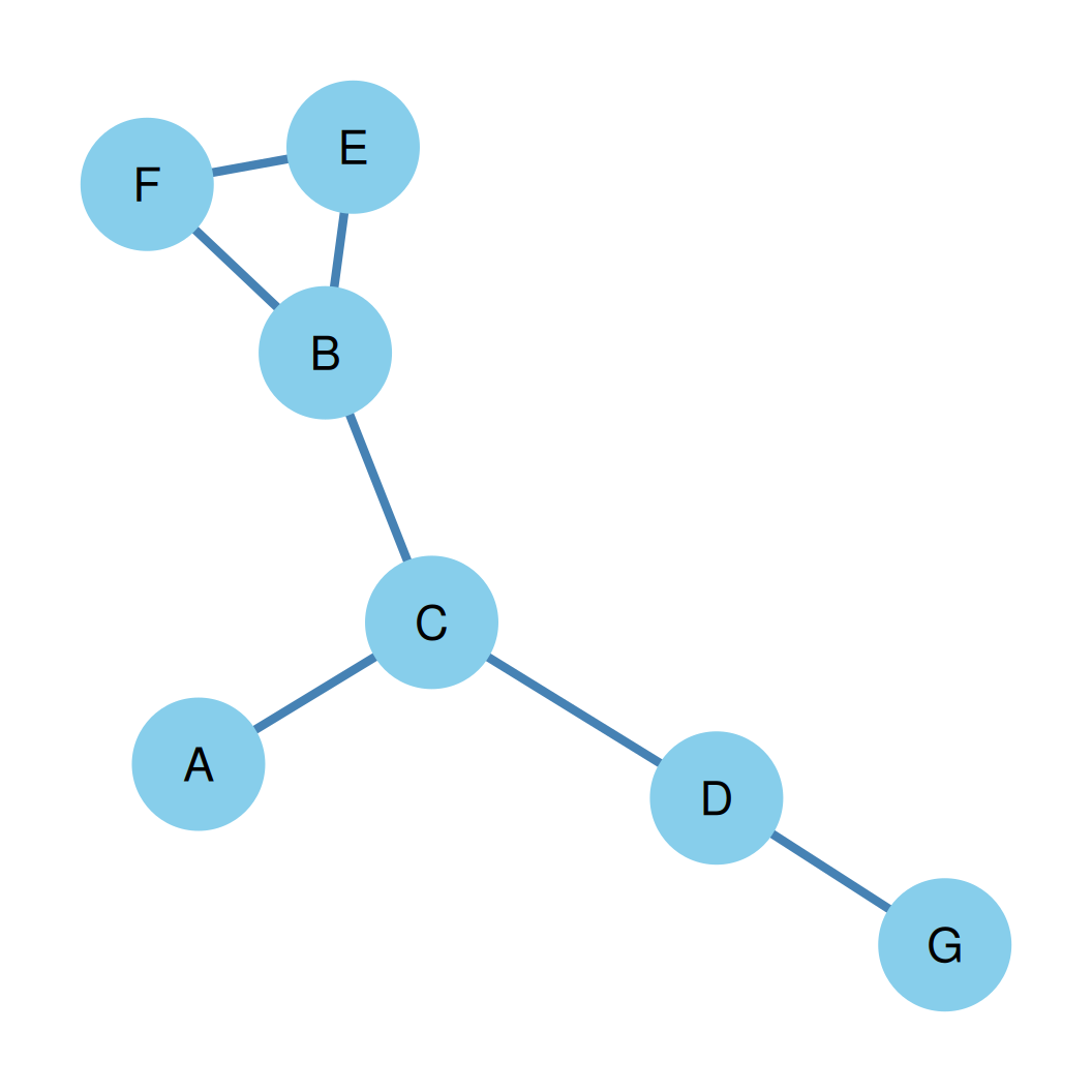
- Let’s look at the undirected graph on the right:
- Order (\(n\)): 7 nodes
- Size (\(m\)): 7 edges
- Maximum possible edges: \[Max(E) = \frac{n(n-1)}{2}\] \[= \frac{7 \times (7-1)}{2} = \frac{7 \times 6}{2}\] \[= \frac{42}{2} = 21\]
Density: Undirected Calculation
- Observed edges (\(m\)): 7 (shown on the right)
- Maximum possible edges: 21
- Density Formula: \[d = \frac{m}{Max(E)} = \frac{7}{21} \approx 0.333\]
- Interpretation:
- Exactly 33.3% of all possible undirected ties are present in this network.
- Equivalently, two randomly chosen nodes have a 33.3% probability of being connected.
Graph Degree Set and Sequence
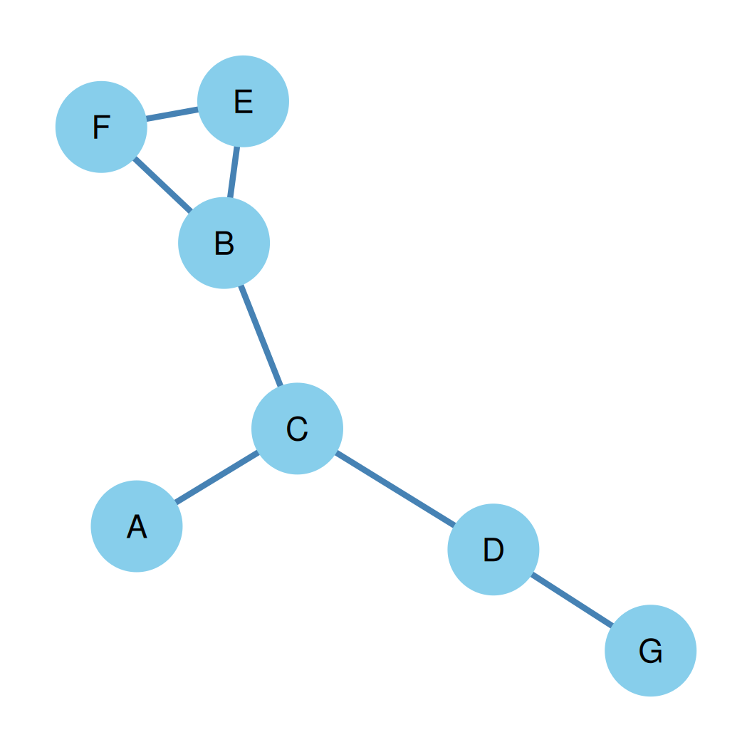
- Graph Degree Set: A list of the degrees of every node in the graph.
- Graph Degree Sequence: The degree set sorted in descending order.
- This provides a “fingerprint” of the graph’s overall connectivity structure.
Degree Set & Sequence: Undirected Example
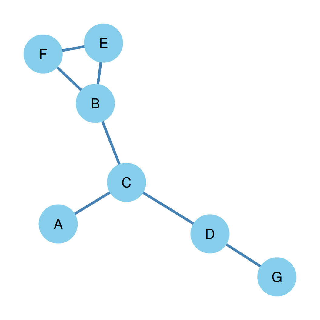
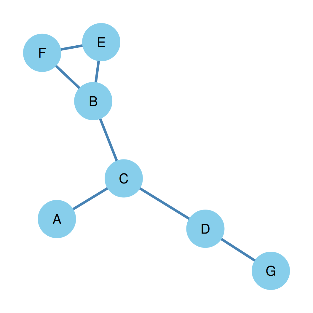
- Degrees: \(k_A=1, k_B=3, k_C=3, k_D=2, k_E=2, k_F=2, k_G=1\) (shown on the right)
- Degree Set (unordered list of node degrees): \[\{1, 3, 3, 2, 2, 2, 1\}\]
- Degree Sequence (sorted degrees): \[(3, 3, 2, 2, 2, 1, 1)\]
Degree Range & Sum
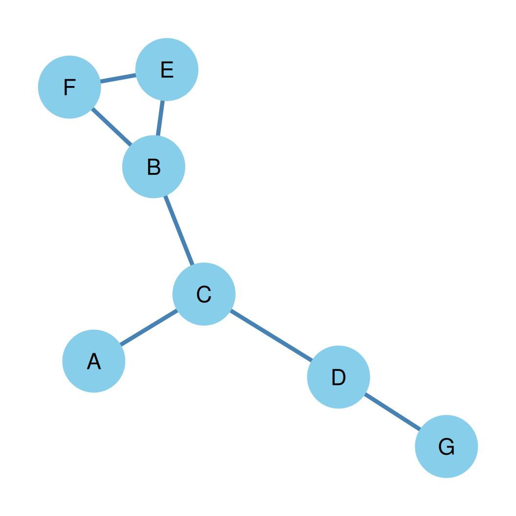
- Maximum Degree (\(k_{max}\)) and Minimum Degree (\(k_{min}\)).
- Degree Range (\(k_r\)): \(k_{max} - k_{min}\).
- Sum of Degrees (\(\sum k_i\)):
- In an undirected graph, this is always twice the number of edges: \(\sum k_i = 2m\).
Degree Range & Sum: Example
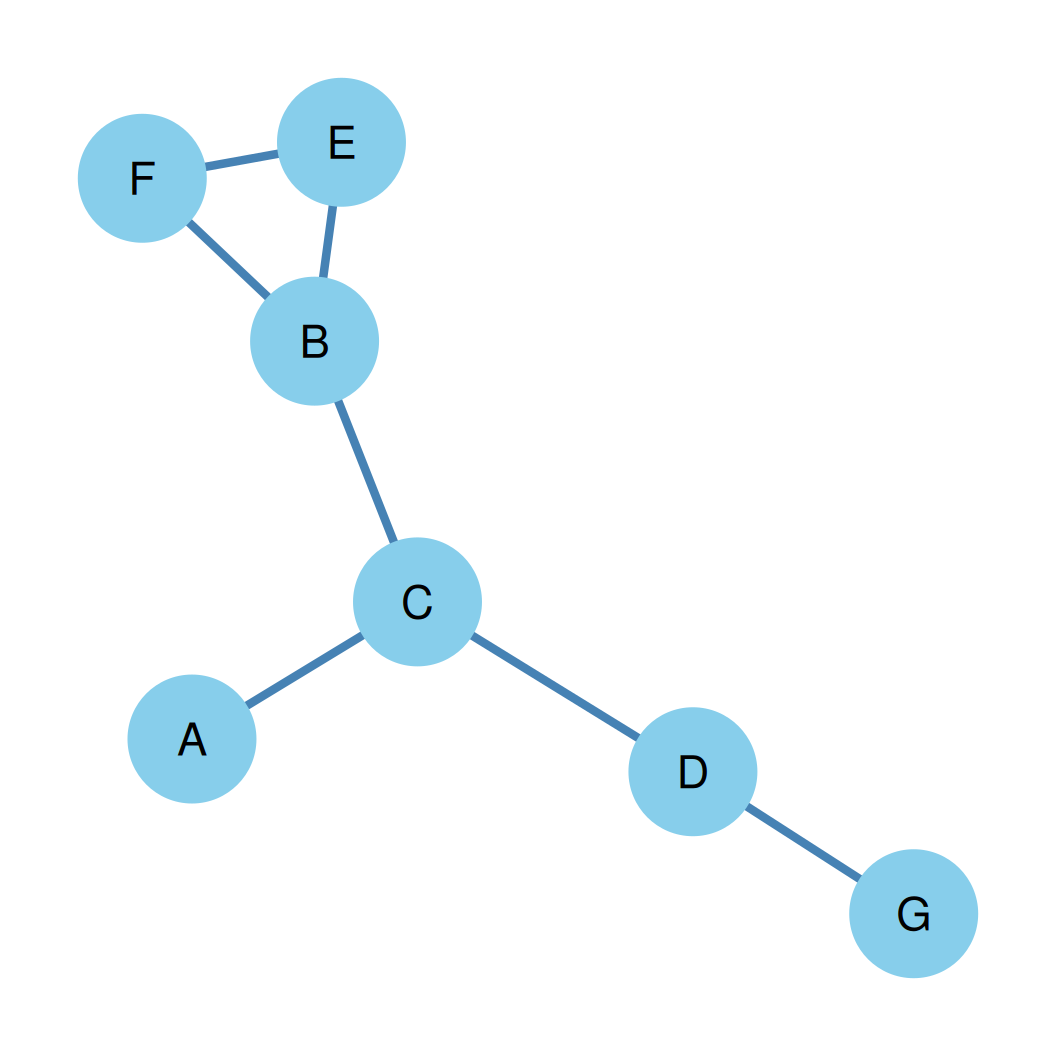
- Degrees: \(k_A=1, k_B=3, k_C=3, k_D=2, k_E=2, k_F=2, k_G=1\) (shown on the right)
- Max & Min Degree:
- \(k_{max} = 3\) (nodes B and C)
- \(k_{min} = 1\) (nodes A and G)
- Degree Range:
- \(k_r = 3 - 1 = 2\)
- Sum of Degrees:
- \(\sum k_i = 1+3+3+2+2+2+1 = 14 = 2m\) (Matches!)
Average Degree
Average Degree (\(\bar{k}\)): The average of all node degrees in the graph.
\[\bar{k} = \frac{1}{n} \sum_{i=1}^{n} k_i = \frac{2m}{n}\]
It represents the expected degree of a randomly chosen node.
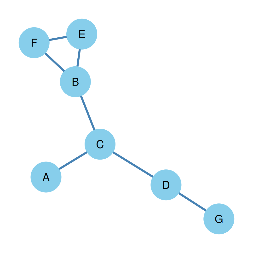
Calculation for the graph on the right:
- Degrees: \(k_A=1, k_B=3, k_C=3, k_D=2, k_E=2, k_F=2, k_G=1\) \[\bar{k} = \frac{\sum k_i}{n} = \frac{1+3+3+2+2+2+1}{7} = \frac{14}{7} = 2.0\]
Connecting Density & Average Degree
- Density (\(d\)) and average degree (\(\bar{k}\)) are intimately related: recall \(d = \frac{2m}{n(n-1)}\) and \(\bar{k} = \frac{2m}{n}\); substituting the latter into the former: \[d = \frac{\bar{k}}{n-1} \qquad \iff \qquad \bar{k} = d(n-1)\]
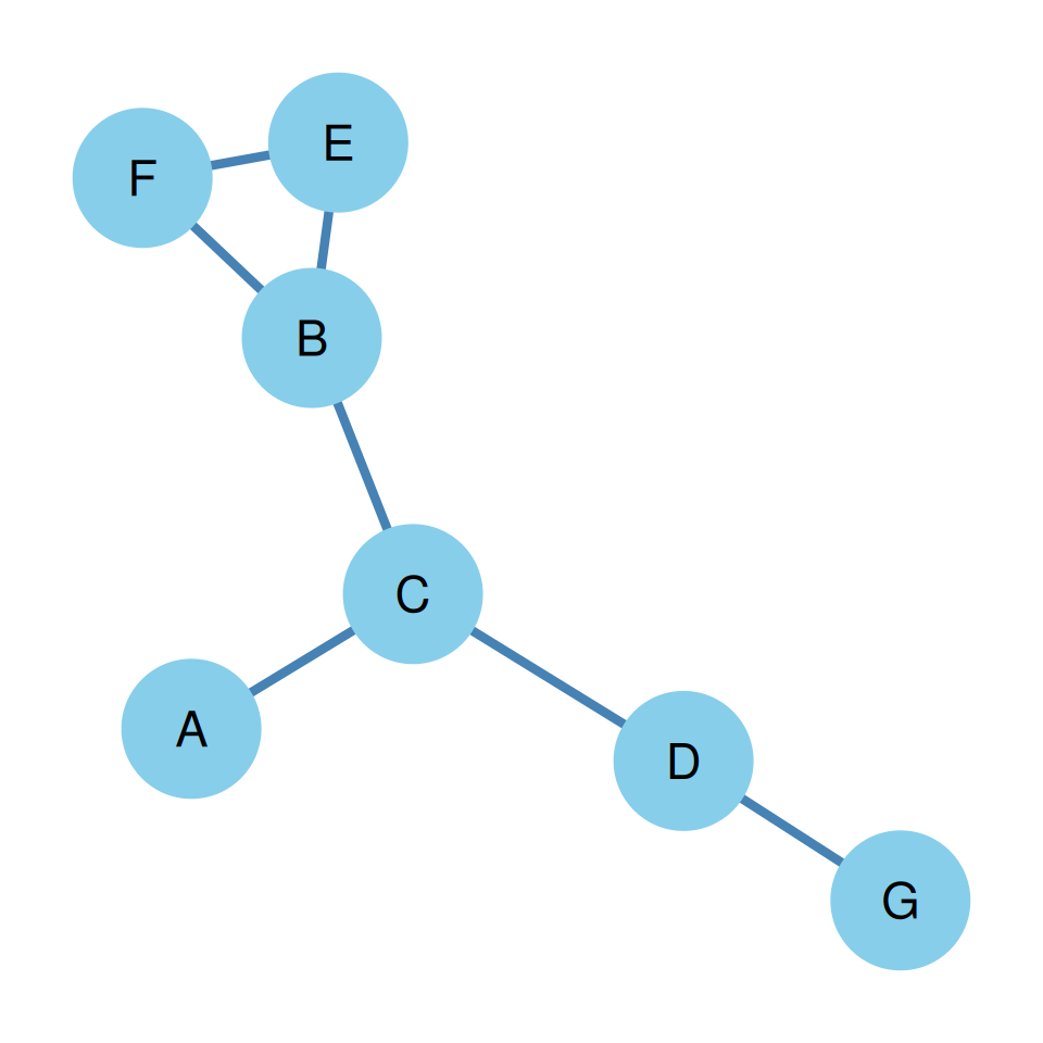
- Numerical example (our graph on the right: \(n = 7\), \(\bar{k} = 2.0\)): \[d = \frac{\bar{k}}{n-1} = \frac{2.0}{7-1} = \frac{2.0}{6} \approx 0.333\]
- This matches the density we computed directly (\(d = 7/21 \approx 0.333\))!
The Density-Degree Connection: Cross-Check
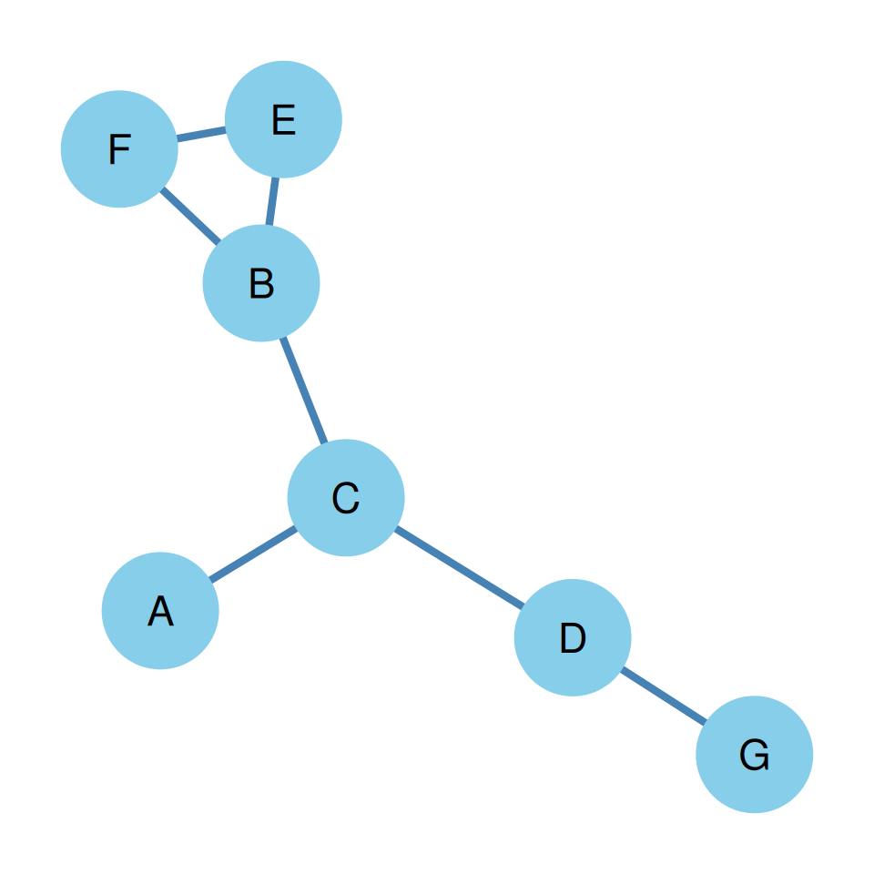
- Cross-Check with Our Graph (\(n = 7\), \(\bar{k} = 2.0\)): \[d = \frac{\bar{k}}{n-1} = \frac{2.0}{7-1} = \frac{2.0}{6} \approx 0.333\]
- Matches the density we computed directly (\(d = 7/21 \approx 0.333\))!
- Directed Case:
- The same identity holds: \(d^d = \frac{\bar{k}}{n-1}\)
Degree Metrics: Basic Example
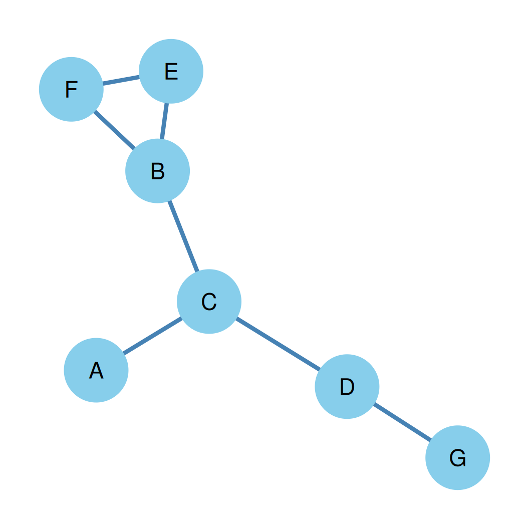
- Node Degrees: \(k_A=1, k_B=3, k_C=3, k_D=2, k_E=2, k_F=2, k_G=1\) (shown on the right)
- Degree Set: \(\{1, 3, 3, 2, 2, 2, 1\}\) (degrees of all nodes in the graph)
- Degree Sequence: \((3, 3, 2, 2, 2, 1, 1)\) (ordered from highest to lowest)
- Degree Sum: \[\sum k_i = 1+3+3+2+2+2+1 = 14 = 2m\]
Degree Metrics: Average Degree
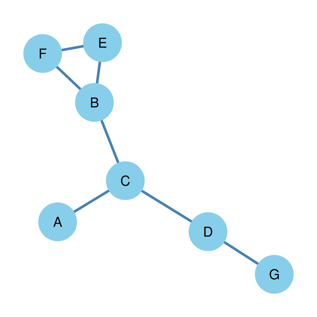
- Degrees: \(k_A=1, k_B=3, k_C=3, k_D=2, k_E=2, k_F=2, k_G=1\) (shown on the right)
- Order (\(n\)): 7 nodes
- Average Degree (\(\bar{k}\)): \[\bar{k} = \frac{\sum k_i}{n} = \frac{14}{7} = 2.0\]
Degree Variance
Degree Variance (\(\sigma^2_k\)): A measure of how much the node degrees vary from the average degree.
\[\sigma^2_k = \frac{1}{n} \sum_{i=1}^{n} (k_i - \bar{k})^2\]
A low variance means less inequality in connectivity (more homogeneous), while a high variance indicates more inequality (more heterogeneous).
Degree Metrics: Degree Variance
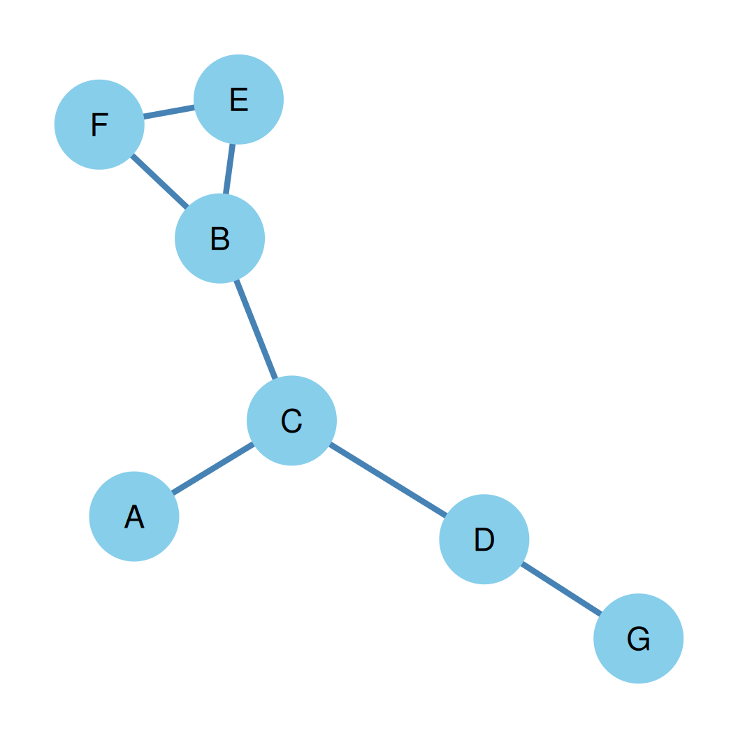
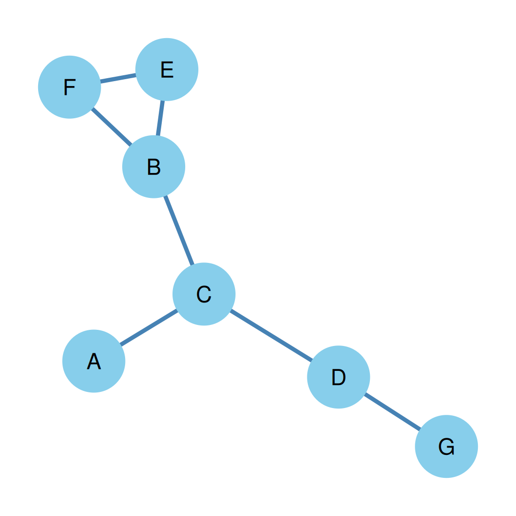
- Degrees: \(k_A=1, k_B=3, k_C=3, k_D=2, k_E=2, k_F=2, k_G=1\) (shown on the right)
- Degree Variance (\(\sigma^2_k\)): \[\sigma^2_k = \frac{\sum (k_i - \bar{k})^2}{n}\]
- Variance Calculation: \[\sigma^2_k = \frac{3 \times (2-2)^2 + 2 \times (3-2)^2 + 2 \times (1-2)^2}{7} = \frac{4}{7} \approx 0.571\]
Regular Graphs
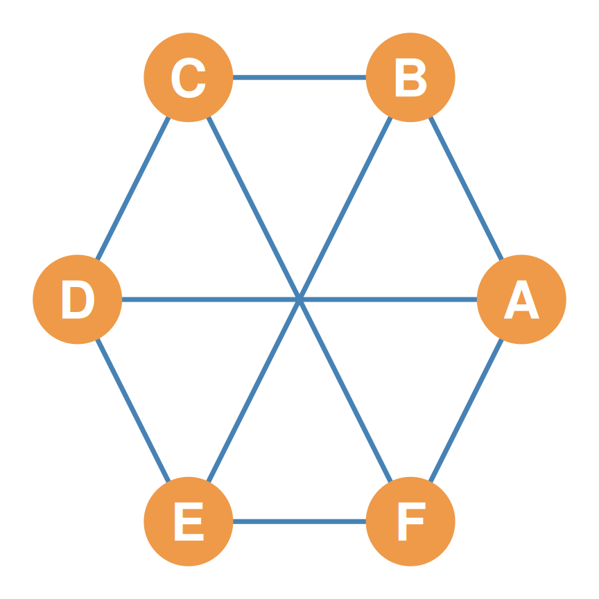
- A regular graph is one where every node has the same degree \(k\) (called \(k\)-regular).
- Since all node degrees are identical to the average, the degree variance is zero (\(\sigma^2_k = 0\)).
- These are rare in real-world social networks but are used as baseline models.
- Example: A 3-regular graph on 6 nodes (shown on the right).
Regular Graphs: Metrics Example
- Node Degrees: \(k_A=3, k_B=3, k_C=3, k_D=3, k_E=3, k_F=3\) (shown on the right)
- Order (\(n\)): 6 nodes
- Average Degree (\(\bar{k}\)): \[\bar{k} = \frac{\sum k_i}{n} = \frac{18}{6} = 3.0\]
Regular Graphs: Variance Example
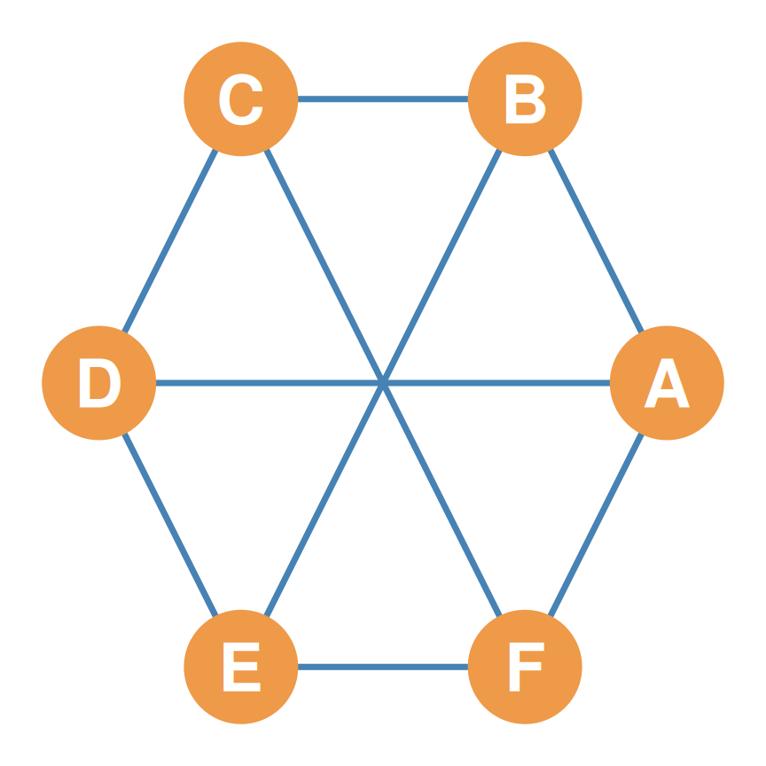
- Average Degree (\(\bar{k}\)): 3.0 (shown on the right)
- Degree Variance (\(\sigma^2_k\)): \[\sigma^2_k = \frac{6 \times (3 - 3)^2}{6} = 0\]
- Conclusion:
- Since every node’s degree matches the average degree, the deviation is zero for all nodes, resulting in zero variance.
Average Nearest Neighbor Degree
- Average Nearest Neighbor Degree (\(\bar{k}_{nn(i)}\)) measures the average degree of node \(i\)’s neighbors.
- Formula: \[\bar{k}_{nn(i)} = \frac{1}{k_i} \sum_{j \in \mathcal{N}(i)} k_j\]
- It tells us whether a node’s connections are, on average, highly connected or peripheral.
Friendship Paradox: Node Calculations
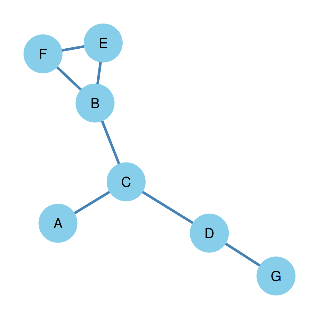
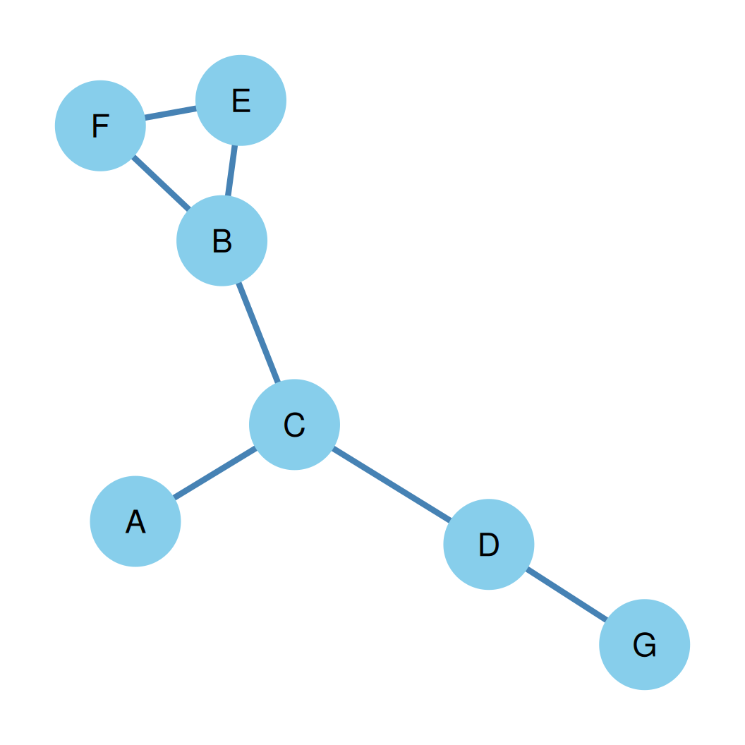
- For the undirected graph shown on the right (average degree \(\bar{k} = 2.0\)):
- Node A (neighbor C): \(\bar{k}_{nn(A)} = \frac{k_C}{1} = \frac{3}{1} = 3.0\)
- Node B (neighbors C, E, F): \(\bar{k}_{nn(B)} = \frac{k_C + k_E + k_F}{3} = \frac{3 + 2 + 2}{3} \approx 2.33\)
- Node C (neighbors A, D, B): \(\bar{k}_{nn(C)} = \frac{k_A + k_D + k_B}{3} = \frac{1 + 2 + 3}{3} = 2.0\)
- Node D (neighbors C, G): \(\bar{k}_{nn(D)} = \frac{k_C + k_G}{2} = \frac{3 + 1}{2} = 2.0\)
- Node E (neighbors B, F): \(\bar{k}_{nn(E)} = \frac{k_B + k_F}{2} = \frac{3 + 2}{2} = 2.5\)
- Node F (neighbors E, B): \(\bar{k}_{nn(F)} = \frac{k_E + k_B}{2} = \frac{2 + 3}{2} = 2.5\)
- Node G (neighbor D): \(\bar{k}_{nn(G)} = \frac{k_D}{1} = \frac{2}{1} = 2.0\)
- Summary of average neighbor degrees:
- \(\bar{k}_{nn} = (3.0, 2.33, 2.0, 2.0, 2.5, 2.5, 2.0)\)
Friendship Paradox: Network Average
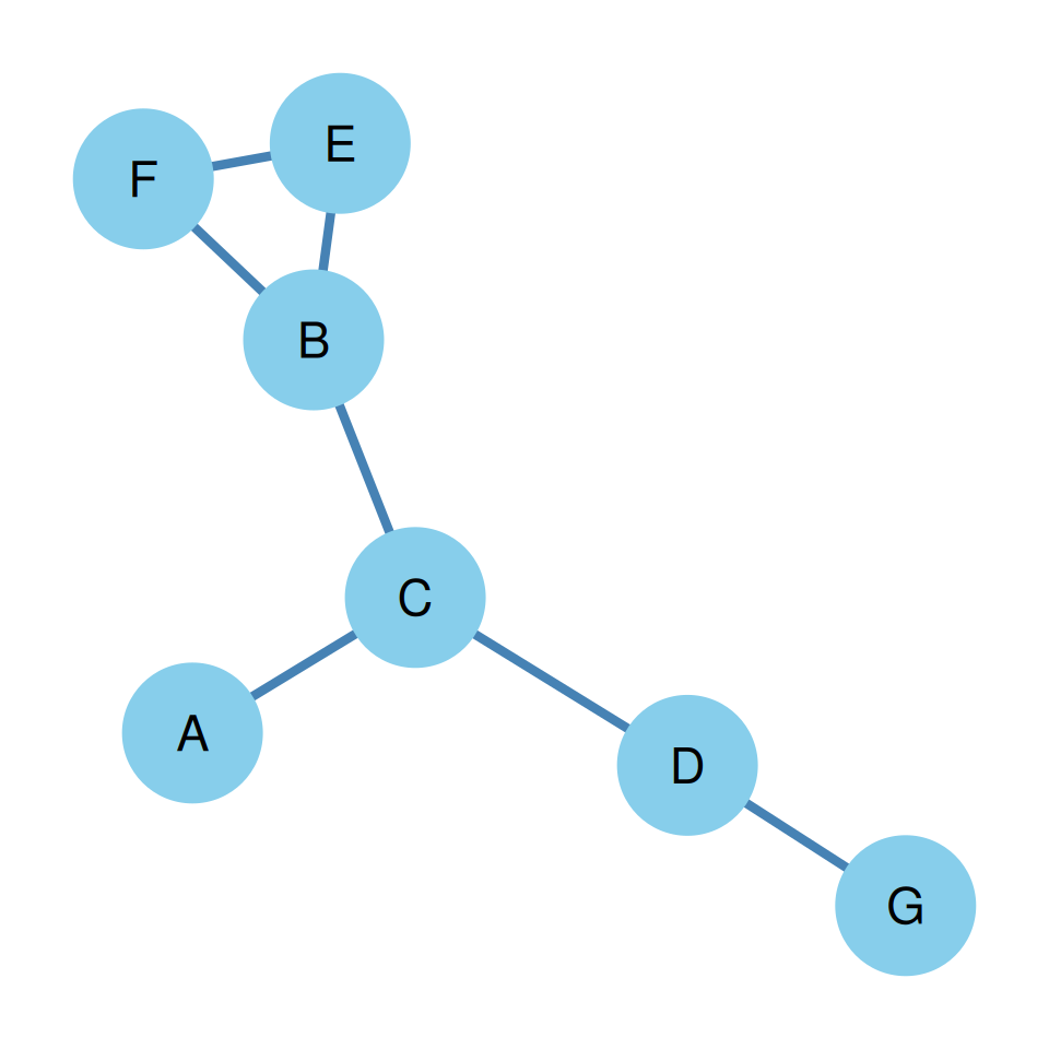
- From the node calculations on the previous slide, the average nearest neighbor degrees are:
- \(\bar{k}_{nn} = (3.0, 2.33, 2.0, 2.0, 2.5, 2.5, 2.0)\)
- Average neighbor degree for the network: \[\text{Mean}(\bar{k}_{nn}) = \frac{3.0 + 2.33 + 2.0 + 2.0 + 2.5 + 2.5 + 2.0}{7} \approx 2.33\]
- Demonstrating the Paradox:
- Average degree of nodes’ neighbors (\(\approx 2.33\)) is greater than the average degree of nodes (\(\bar{k} = 2.0\)).
Graphicality: Concrete Examples
- Graphical Sequence: \(\mathbf{d} = (4, 3, 3, 2, 2, 1, 1)\) with \(n = 7\)
- Sum is \(16\) (even). Max degree is \(4 \le 6\).
- A real simple graph can easily be constructed with these degrees (shown on the right).
- Non-Graphical Sequence (Odd Sum Violation): \(\mathbf{d} = (4, 3, 3, 3, 2, 1, 1)\) with \(n = 7\)
- Sum is \(17\) (odd). Violates Handshake Lemma.
- No simple graph can ever have this sequence.
- Non-Graphical Sequence (Degree Bound Violation): \(\mathbf{d} = (7, 2, 2, 1)\) with \(n = 4\)
- Max degree is \(7\), which is greater than \(n-1 = 3\).
- A node in a 4-person group cannot have 7 unique friends!