Advanced Network Matrices
Beyond the Adjacency Matrix
Step 1: Filling Row A (Actor A’s Reachability)
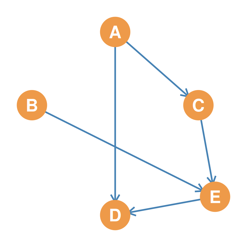
Let’s trace which nodes can be reached by starting a directed walk at node A.
| A | B | C | D | E | |
|---|---|---|---|---|---|
| A | -- | 0 | 1 | 1 | 1 |
| B | ? | -- | ? | ? | ? |
| C | ? | ? | -- | ? | ? |
| D | ? | ? | ? | -- | ? |
| E | ? | ? | ? | ? | -- |
- B? No (\(d^r_{AB} = 0\)) — no arrow points into B.
- C? Yes (\(d^r_{AC} = 1\)) — direct link \(A \rightarrow C\).
- D? Yes (\(d^r_{AD} = 1\)) — direct link \(A \rightarrow D\).
- E? Yes (\(d^r_{AE} = 1\)) — path \(A \rightarrow C \rightarrow E\).
Step 2: Filling Row B (Actor B’s Reachability)
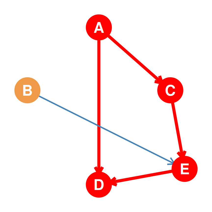
Let’s trace which nodes can be reached by starting a directed walk at node B.
| A | B | C | D | E | |
|---|---|---|---|---|---|
| A | -- | 0 | 1 | 1 | 1 |
| B | 0 | -- | 0 | 1 | 1 |
| C | ? | ? | -- | ? | ? |
| D | ? | ? | ? | -- | ? |
| E | ? | ? | ? | ? | -- |
- A or C? No (\(d^r_{BA} = d^r_{BC} = 0\)) — the only arrow out of E is \(E \rightarrow D\), a dead end.
- D? Yes (\(d^r_{BD} = 1\)) — path \(B \rightarrow E \rightarrow D\), length 2.
- E? Yes (\(d^r_{BE} = 1\)) — direct link \(B \rightarrow E\).
Step 3: Filling Row C (Actor C’s Reachability)
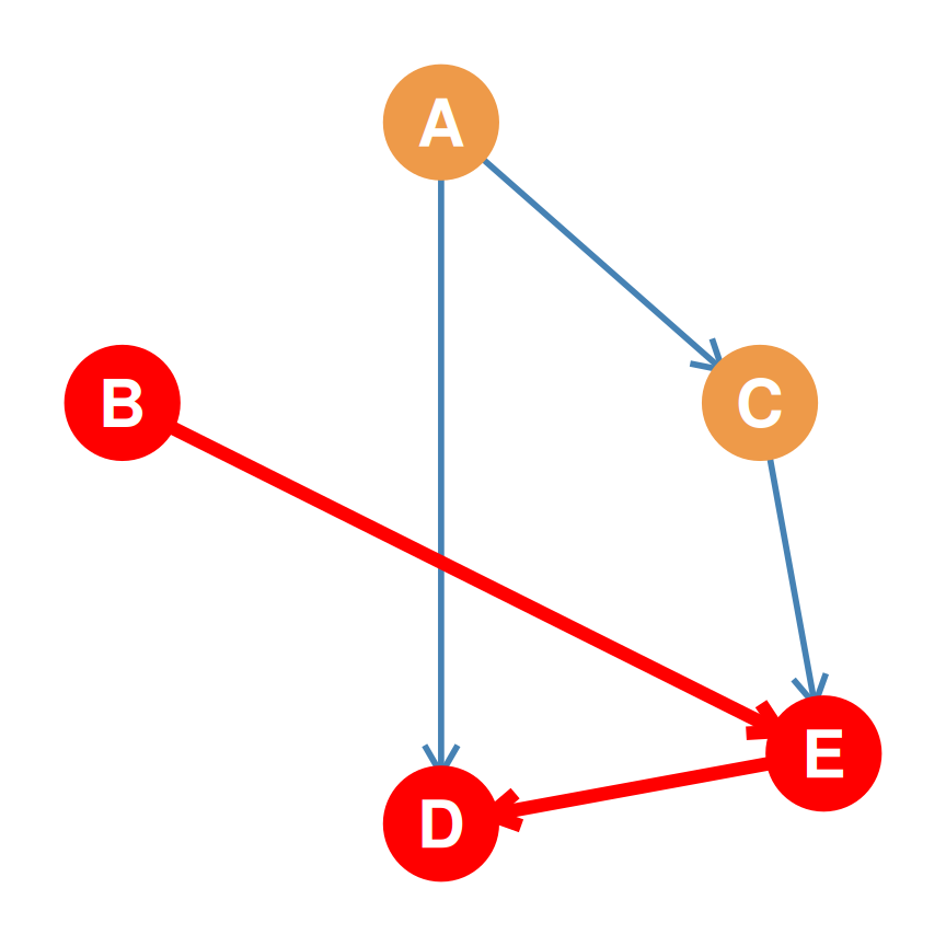
Same trace for node C — and a pattern emerges: nothing ever points into A or B, the two pure sources.
| A | B | C | D | E | |
|---|---|---|---|---|---|
| A | -- | 0 | 1 | 1 | 1 |
| B | 0 | -- | 0 | 1 | 1 |
| C | 0 | 0 | -- | 1 | 1 |
| D | ? | ? | ? | -- | ? |
| E | ? | ? | ? | ? | -- |
- A or B? No (\(d^r_{CA} = d^r_{CB} = 0\)) — no directed path can end at a pure source.
- D? Yes (\(d^r_{CD} = 1\)) — path \(C \rightarrow E \rightarrow D\), length 2.
- E? Yes (\(d^r_{CE} = 1\)) — direct link \(C \rightarrow E\).
Step 4: Filling Rows D and E
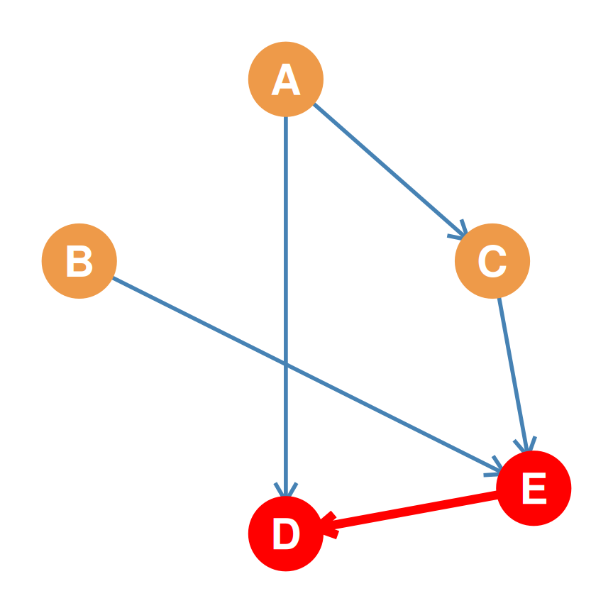
The last two rows are the quickest — and the most informative.
| A | B | C | D | E | |
|---|---|---|---|---|---|
| A | -- | 0 | 1 | 1 | 1 |
| B | 0 | -- | 0 | 1 | 1 |
| C | 0 | 0 | -- | 1 | 1 |
| D | 0 | 0 | 0 | -- | 0 |
| E | 0 | 0 | 0 | 1 | -- |
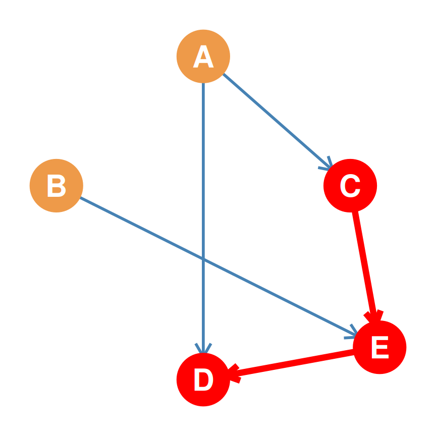
- Row D: D has no outgoing arrows, so its row is all \(0\)s — the pure receiver: everyone reaches D, D reaches no one.
- Row E: E’s only arrow is \(E \rightarrow D\), so E reaches exactly one node: D.
Step 5: Completed Reachability Matrix
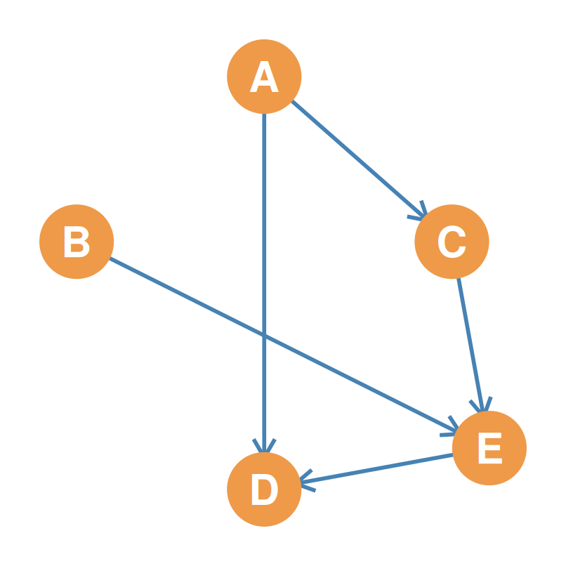
Tracing every row fills the matrix — and the completed matrix reveals each node’s role at a glance.
| A | B | C | D | E | |
|---|---|---|---|---|---|
| A | -- | 0 | 1 | 1 | 1 |
| B | 0 | -- | 0 | 1 | 1 |
| C | 0 | 0 | -- | 1 | 1 |
| D | 0 | 0 | 0 | -- | 0 |
| E | 0 | 0 | 0 | 1 | -- |
- Unreached Sources (A, B): columns A and B are all \(0\)s — no one reaches them.
- Pure Receiver (D): row D is all \(0\)s — D reaches no one, while everyone reaches D.
Pairwise Weakly Connected
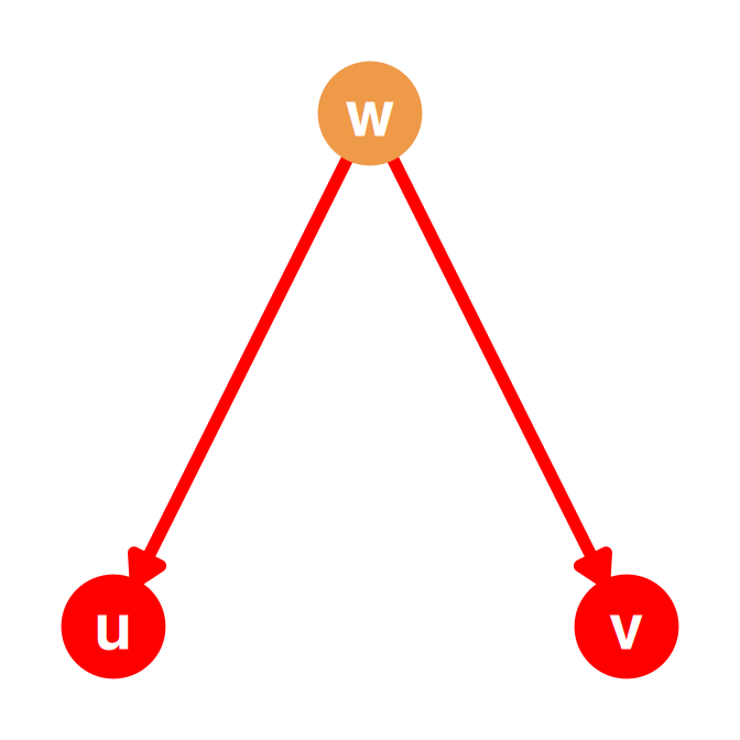
- Example: \(w\) sends to both members of the pair \(u, v\) (red).
- Definition: Nodes \(u\) and \(v\) are connected by at least one semipath (connected if we ignore the arrow directions).
- Sociological Meaning: They are part of the same general network, but there is no directed path starting from either node that can reach the other.
- In the example: \(u\) and \(v\) are linked only through \(w\), and only once we ignore the arrows — no path starts at \(u\) or \(v\) at all.
Pairwise Unilaterally Connected
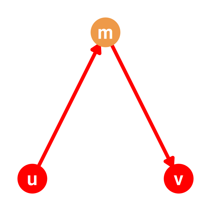
- Example: \(u\) reaches \(v\) via \(m\); \(v\) cannot reach back.
- Definition: A directed path exists from \(u \rightarrow v\) OR from \(v \rightarrow u\) (one-way reachability).
- Sociological Meaning: Information or influence can flow from one person to the other, but not in both directions (no mutual exchange).
- In the example: the directed path \(u \rightarrow m \rightarrow v\) runs one way only.
Pairwise Strongly Connected
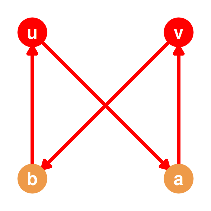
- Example: \(u\) reaches \(v\) via \(a\); \(v\) reaches \(u\) via \(b\).
- Definition: A directed path exists from \(u \rightarrow v\) AND from \(v \rightarrow u\) (mutual reachability).
- Sociological Meaning: Both nodes can reach each other, but the paths in each direction may use completely different intermediate nodes or channels.
- In the example: the two directions travel through different intermediaries (\(a\) vs. \(b\)).
Pairwise Recursively Connected
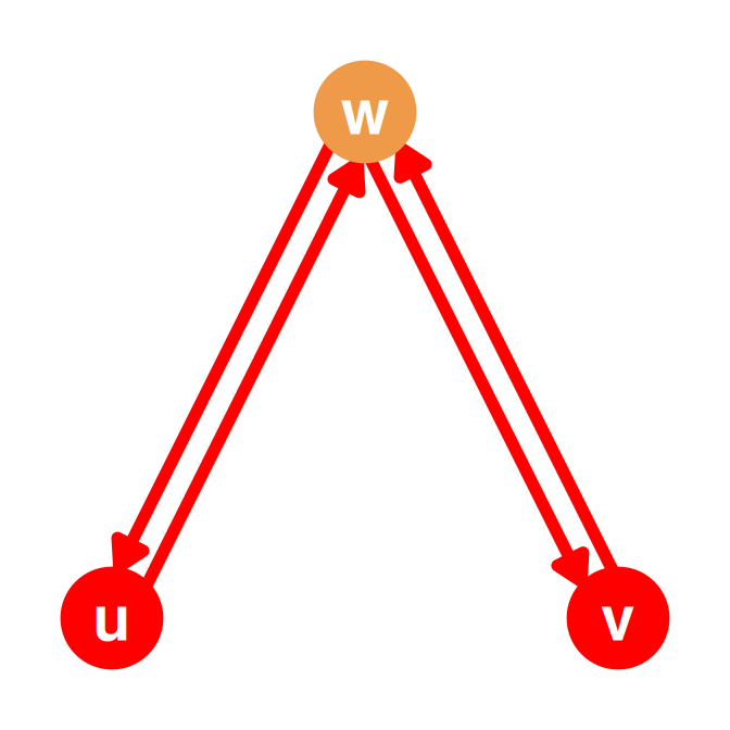
- Example: \(u\) and \(v\) reach each other through the same intermediary \(w\).
- Definition: A directed path exists from \(u \rightarrow v\) and \(v \rightarrow u\), AND the directed path in both directions shares the exact same set of intermediate nodes (sharing both vertices and edges).
- Sociological Meaning: The relationship can be traversed back-and-forth along the same closed, mutually symmetric cycle.
- In the example: both directions use the same intermediary \(w\) and the same reciprocated ties \(u \leftrightarrow w \leftrightarrow v\).
Case 1: Strongly Connected Graphs
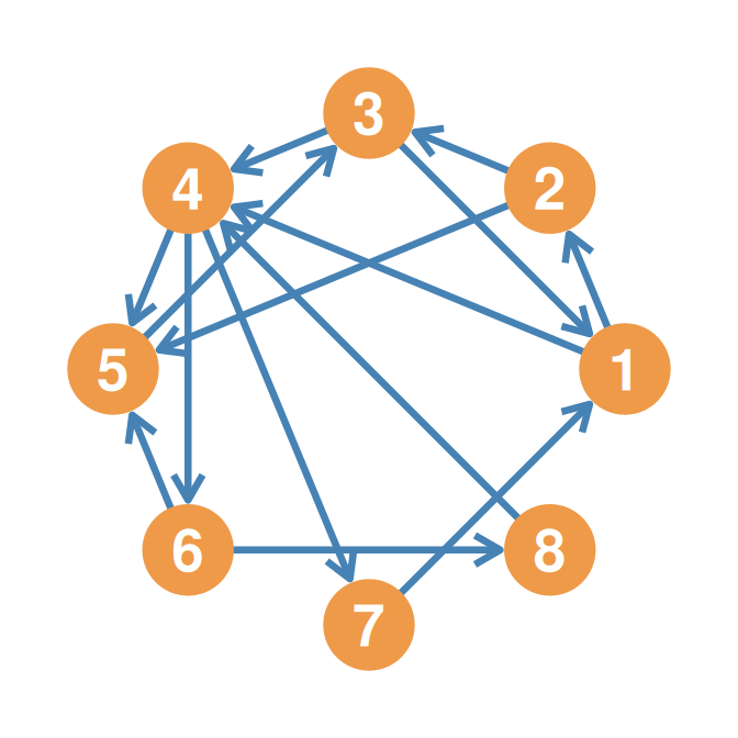
- Strongly connected: every pair of nodes is mutually reachable.
- 8-Node Example (Left): interlocking directed cycles thread through all eight nodes.
| 1 | 2 | 3 | 4 | 5 | 6 | 7 | 8 | |
|---|---|---|---|---|---|---|---|---|
| 1 | – | 1 | 1 | 1 | 1 | 1 | 1 | 1 |
| 2 | 1 | – | 1 | 1 | 1 | 1 | 1 | 1 |
| 3 | 1 | 1 | – | 1 | 1 | 1 | 1 | 1 |
| 4 | 1 | 1 | 1 | – | 1 | 1 | 1 | 1 |
| 5 | 1 | 1 | 1 | 1 | – | 1 | 1 | 1 |
| 6 | 1 | 1 | 1 | 1 | 1 | – | 1 | 1 |
| 7 | 1 | 1 | 1 | 1 | 1 | 1 | – | 1 |
| 8 | 1 | 1 | 1 | 1 | 1 | 1 | 1 | – |
- No Zeros: everyone can reach everyone, so the reachability matrix is the all-ones matrix!
- Trace: \(D^r_{18} = 1\) via \(1 \rightarrow 4 \rightarrow 6 \rightarrow 8\).
Case 2: Unilaterally Connected Graphs
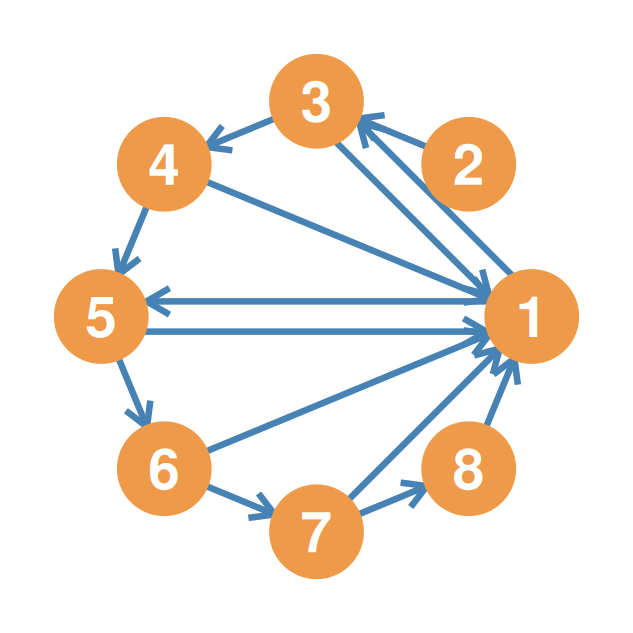
- Unilaterally connected: at least one directed path between every pair, but not necessarily both ways.
- Some Zeros: Column 2 is all \(0\)s — node 2 is a transmitter (sends to everyone, receives from no one).
- No Symmetric Zeros: for any pair \(\{u, v\}\), at least one direction is always \(1\).
| 1 | 2 | 3 | 4 | 5 | 6 | 7 | 8 | |
|---|---|---|---|---|---|---|---|---|
| 1 | – | 0 | 1 | 1 | 1 | 1 | 1 | 1 |
| 2 | 1 | – | 1 | 1 | 1 | 1 | 1 | 1 |
| 3 | 1 | 0 | – | 1 | 1 | 1 | 1 | 1 |
| 4 | 1 | 0 | 1 | – | 1 | 1 | 1 | 1 |
| 5 | 1 | 0 | 1 | 1 | – | 1 | 1 | 1 |
| 6 | 1 | 0 | 1 | 1 | 1 | – | 1 | 1 |
| 7 | 1 | 0 | 1 | 1 | 1 | 1 | – | 1 |
| 8 | 1 | 0 | 1 | 1 | 1 | 1 | 1 | – |
- Trace: \(D^r_{25} = 1\) via \(2 \rightarrow 3 \rightarrow 4 \rightarrow 5\) — but \(D^r_{52} = 0\), since no arrow ever points into node 2.
Case 3: Weakly Connected Graphs
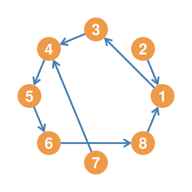
- Mutually Unreachable Pair:
- Node 2 can’t reach 7 (\(D^r_{27}=0\)), and Node 7 can’t reach 2 (\(D^r_{72}=0\)).
- This symmetric zero (\(D^r_{27} = D^r_{72} = 0\)) proves they are mutually unreachable, making the graph weakly connected.
| 1 | 2 | 3 | 4 | 5 | 6 | 7 | 8 | |
|---|---|---|---|---|---|---|---|---|
| 1 | – | 0 | 1 | 1 | 1 | 1 | 0 | 1 |
| 2 | 1 | – | 1 | 1 | 1 | 1 | 0 | 1 |
| 3 | 1 | 0 | – | 1 | 1 | 1 | 0 | 1 |
| 4 | 1 | 0 | 1 | – | 1 | 1 | 0 | 1 |
| 5 | 1 | 0 | 1 | 1 | – | 1 | 0 | 1 |
| 6 | 1 | 0 | 1 | 1 | 1 | – | 0 | 1 |
| 7 | 1 | 0 | 1 | 1 | 1 | 1 | – | 1 |
| 8 | 1 | 0 | 1 | 1 | 1 | 1 | 0 | – |
- Trace: \(D^r_{71} = 1\) via \(7 \rightarrow 4 \rightarrow 5 \rightarrow 6 \rightarrow 8 \rightarrow 1\).
Decomposing Directed Components
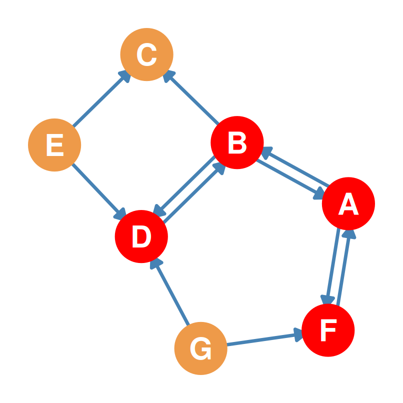
- A graph that fails even weak connectivity breaks into multiple disconnected pieces; our example holds together weakly but decomposes further once direction matters:
- Weakly Connected Components (WCCs):
- Subgraphs connected when ignoring edge directions.
- Yields one WCC containing all 7 nodes: \(\{A, B, C, D, E, F, G\}\).
- Strongly Connected Components (SCCs):
- Subgraphs where every pair is mutually reachable.
- Yields four SCCs:
- \(\{A, B, D, F\}\) (the core “rumor mill”, highlighted in red).
- Singletons: \(\{C\}\), \(\{E\}\), \(\{G\}\).
| A | B | C | D | E | F | G | |
|---|---|---|---|---|---|---|---|
| A | -- | 1 | 1 | 1 | 0 | 1 | 0 |
| B | 1 | -- | 1 | 1 | 0 | 1 | 0 |
| C | 0 | 0 | -- | 0 | 0 | 0 | 0 |
| D | 1 | 1 | 1 | -- | 0 | 1 | 0 |
| E | 1 | 1 | 1 | 1 | -- | 1 | 0 |
| F | 1 | 1 | 1 | 1 | 0 | -- | 0 |
| G | 1 | 1 | 1 | 1 | 0 | 1 | -- |
- Red block: rows/cols \(A, B, D, F\) are all 1s — every pair mutually reachable.
- \(E\) and \(G\) reach the core, but nothing reaches them; \(C\) reaches nothing at all.
Measuring Graph Connectedness (\(C\))
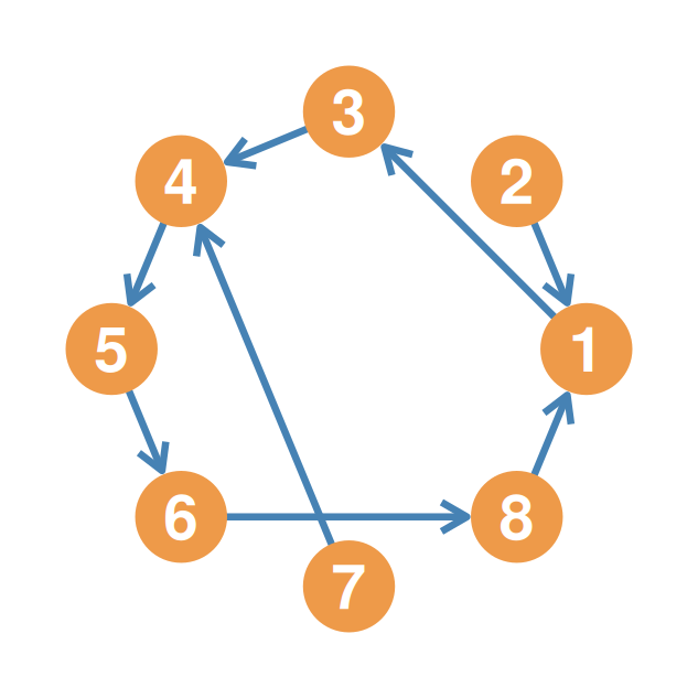
- Graph Connectedness (\(C\)) measures the overall capacity of a network to facilitate connections.
- It is defined as the density of the reachability matrix (excluding diagonal cells):
- \[C = \frac{\sum_{i \neq j} D^r_{ij}}{N(N-1)}\]
Reachability Density
| Value | Meaning |
|---|---|
| \(C = 1.0\) | Strongly connected (all-ones matrix). |
| \(C < 1.0\) | Unilaterally or weakly connected (has zeros). |
| \(C = 0.0\) | Completely disconnected (all zeros). |
Graph Connectedness: Worked Example
| 1 | 2 | 3 | 4 | 5 | 6 | 7 | 8 | |
|---|---|---|---|---|---|---|---|---|
| 1 | -- | 0 | 1 | 1 | 1 | 1 | 0 | 1 |
| 2 | 1 | -- | 1 | 1 | 1 | 1 | 0 | 1 |
| 3 | 1 | 0 | -- | 1 | 1 | 1 | 0 | 1 |
| 4 | 1 | 0 | 1 | -- | 1 | 1 | 0 | 1 |
| 5 | 1 | 0 | 1 | 1 | -- | 1 | 0 | 1 |
| 6 | 1 | 0 | 1 | 1 | 1 | -- | 0 | 1 |
| 7 | 1 | 0 | 1 | 1 | 1 | 1 | -- | 1 |
| 8 | 1 | 0 | 1 | 1 | 1 | 1 | 0 | -- |
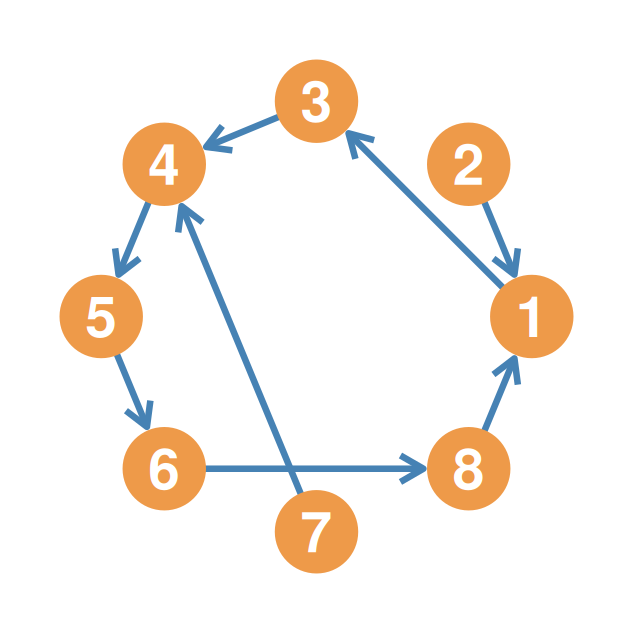
- For our weakly connected 8-node graph (left):
- Total possible off-diagonal cells: \(8(7) = 56\).
- The \(0\) cells sit in the highlighted columns 2 and 7: \(7 + 7 = 14\) zeros.
- So the sum of all \(1\) cells is \(56 - 14 = 42\).
- \[C = \frac{42}{56} = 0.75\]
- The only mutually unreachable pair is \(\{2, 7\}\) — two pure transmitters, with \(D^r_{27} = D^r_{72} = 0\).
Step 1: Distance Matrix (Undirected) - Adjacencies
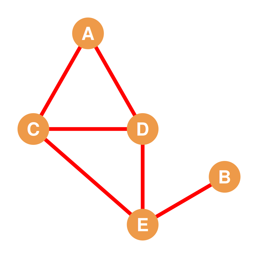
We now switch to a new undirected 5-node example. Nodes with direct connections get a geodesic distance of 1.0.
| A | B | C | D | E | |
|---|---|---|---|---|---|
| A | 0 | ? | 1 | 1 | ? |
| B | ? | 0 | ? | ? | 1 |
| C | 1 | ? | 0 | 1 | 1 |
| D | 1 | ? | 1 | 0 | 1 |
| E | ? | 1 | 1 | 1 | 0 |
- Symmetrical connections \(a_{AC} = a_{CA} = 1.0\), etc.
- Diagonals are initialized to 0 because \(d(v, v) = 0\).
Step 2: Distance Matrix (Undirected) - Paths of Length 2
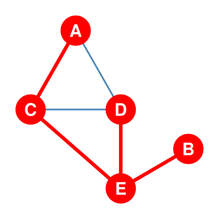
For non-adjacent nodes, we calculate the length of the shortest path connecting them.
| A | B | C | D | E | |
|---|---|---|---|---|---|
| A | 0 | ? | 1 | 1 | 2 |
| B | ? | 0 | 2 | 2 | 1 |
| C | 1 | 2 | 0 | 1 | 1 |
| D | 1 | 2 | 1 | 0 | 1 |
| E | 2 | 1 | 1 | 1 | 0 |
- B to C: Shortest path is \(B \rightarrow E \rightarrow C\) (length 2).
- B to D: Shortest path is \(B \rightarrow E \rightarrow D\) (length 2).
- A to E: Shortest path is \(A \rightarrow C \rightarrow E\) (length 2).
Step 3: Distance Matrix (Undirected) - Paths of Length 3
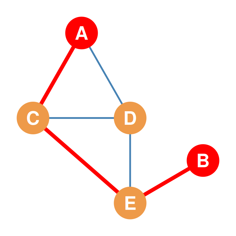
We compute the remaining non-adjacent pair, representing the maximum distance in the graph.
| A | B | C | D | E | |
|---|---|---|---|---|---|
| A | 0 | 3 | 1 | 1 | 2 |
| B | 3 | 0 | 2 | 2 | 1 |
| C | 1 | 2 | 0 | 1 | 1 |
| D | 1 | 2 | 1 | 0 | 1 |
| E | 2 | 1 | 1 | 1 | 0 |
- A to B: Shortest path is \(A \rightarrow C \rightarrow E \rightarrow B\) (length 3).
- This completed matrix is perfectly symmetric!
Step 4: Distance Matrix (Directed) - Paths & Connections
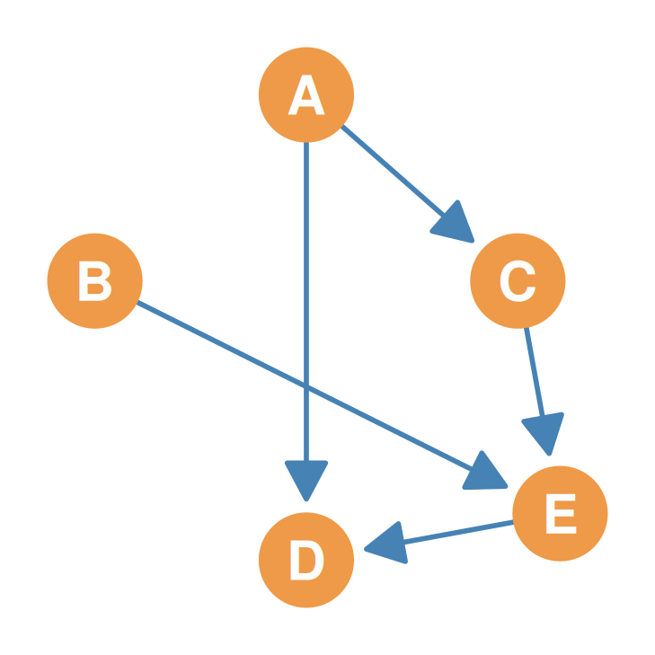
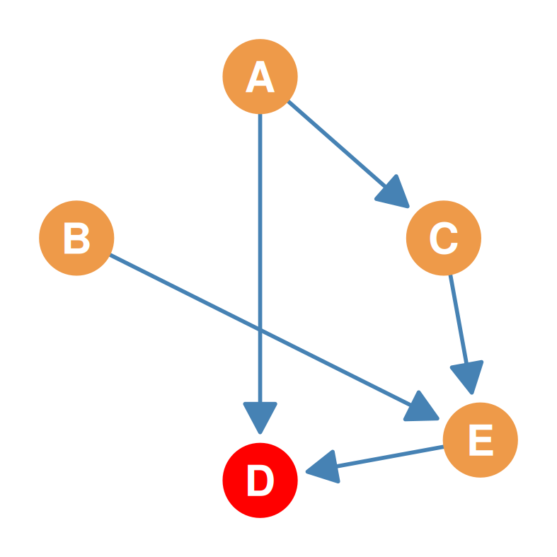
For directed graphs, we follow the same process but respect the arrows (Sender \(\rightarrow\) Receiver) — back on the same digraph we used for reachability in Part 1.
| A | B | C | D | E | |
|---|---|---|---|---|---|
| A | 0 | ? | 1 | 1 | 2 |
| B | ? | 0 | ? | 2 | 1 |
| C | ? | ? | 0 | 2 | 1 |
| D | ? | ? | ? | 0 | ? |
| E | ? | ? | ? | 1 | 0 |
- Direct links: \(A \rightarrow C = 1\), \(A \rightarrow D = 1\), \(B \rightarrow E = 1\), \(C \rightarrow E = 1\), \(E \rightarrow D = 1\).
- Path of length 2: \(A \rightarrow C \rightarrow E\) (length 2), \(B \rightarrow E \rightarrow D\) (length 2), \(C \rightarrow E \rightarrow D\) (length 2).
Step 5: Distance Matrix (Directed) - Unreachable Pairs
If a node \(i\) cannot reach node \(j\) via any directed path, their geodesic distance is Infinity (\(\infty\)).
| A | B | C | D | E | |
|---|---|---|---|---|---|
| A | 0 | \(\infty\) | 1 | 1 | 2 |
| B | \(\infty\) | 0 | \(\infty\) | 2 | 1 |
| C | \(\infty\) | \(\infty\) | 0 | 2 | 1 |
| D | \(\infty\) | \(\infty\) | \(\infty\) | 0 | \(\infty\) |
| E | \(\infty\) | \(\infty\) | \(\infty\) | 1 | 0 |
- Unreachable: e.g., \(B\) can’t reach \(A\), so \(d^g_{BA} = \infty\).
- Pure Sink (D): Row D is full of \(\infty\) cells since node D can’t reach anyone.
- Check vs. Part 1: same digraph as Part 1 — every \(\infty\) here sits on a \(0\) in \(\mathbf{D^r}\).
Visualizing Node Eccentricity
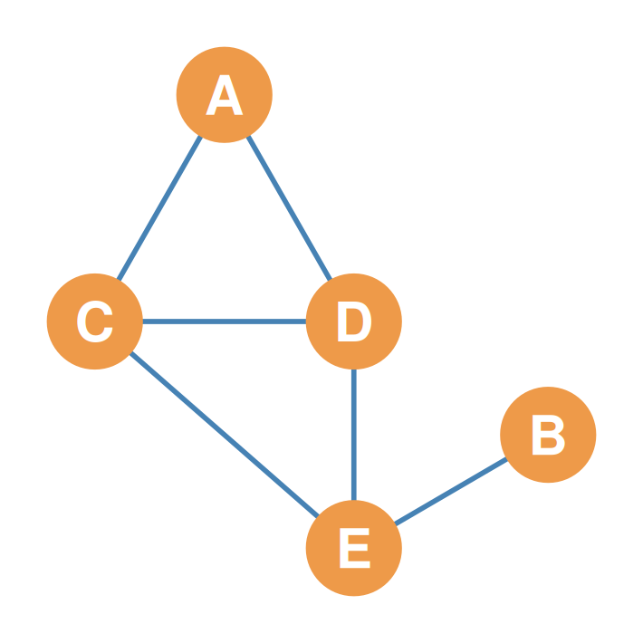
- We return to our undirected 5-node example (Steps 1–3 distance matrix): eccentricity is the maximum value in each row (excluding diagonal 0s).
| A | B | C | D | E | Row Max (\(e\)) | |
|---|---|---|---|---|---|---|
| A | 0 | 3 | 1 | 1 | 2 | \(e(A) = 3\) |
| B | 3 | 0 | 2 | 2 | 1 | \(e(B) = 3\) |
| C | 1 | 2 | 0 | 1 | 1 | \(e(C) = 2\) |
| D | 1 | 2 | 1 | 0 | 1 | \(e(D) = 2\) |
| E | 2 | 1 | 1 | 1 | 0 | \(e(E) = 2\) |
- Graph Diameter (\(d\)): The maximum eccentricity across all nodes is 3 (\(d = 3\)).
- Nodes C, D, E are the most central (closest “worst-case” distance of 2).
Step-by-Step: Overlap of \(A\) and \(C\)
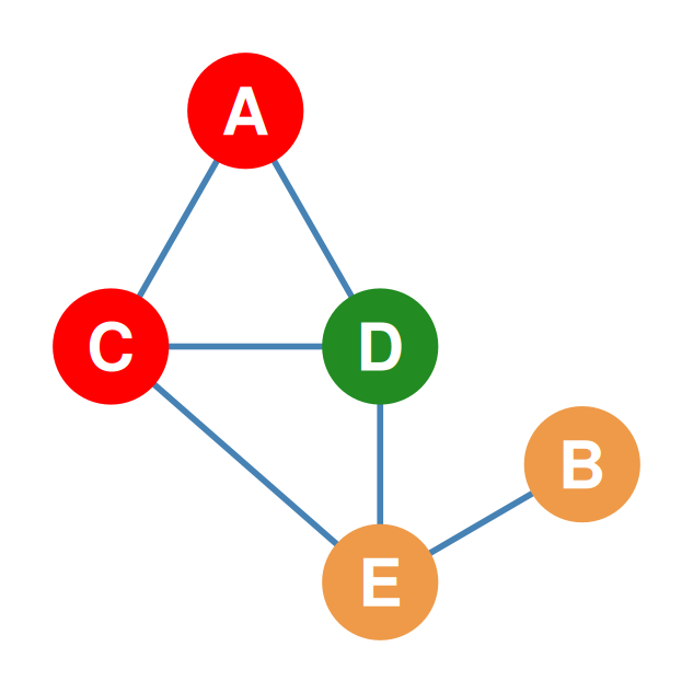
- Focal pair in red, shared neighbors in green.
| A | B | C | D | E | |
|---|---|---|---|---|---|
| A | -- | 0.00 | 0.25 | 0.25 | 0.67 |
| B | 0.00 | -- | 0.33 | 0.33 | 0.00 |
| C | 0.25 | 0.33 | -- | 0.50 | 0.20 |
| D | 0.25 | 0.33 | 0.50 | -- | 0.20 |
| E | 0.67 | 0.00 | 0.20 | 0.20 | -- |
- Diagonal (
--): \(J_{ii}\) is trivially 1.
- \(\mathcal{N}(A) = \{C, D\}\) (\(k_A = 2\))
- \(\mathcal{N}(C) = \{A, D, E\}\) (\(k_C = 3\))
- Intersection: \(\mathcal{N}(A) \cap \mathcal{N}(C) = \{D\}\) — node \(D\) (green) is connected to both. Cardinality 1.
- Union: \(\mathcal{N}(A) \cup \mathcal{N}(C) = \{A, C, D, E\}\). Cardinality 4.
- Overlap: \[O_{AC} = \frac{1}{4} = 0.25\]
Step-by-Step: Overlap of \(C\) and \(D\)
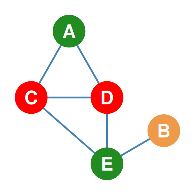
- Two shared neighbors this time: \(A\) and \(E\) (green).
| A | B | C | D | E | |
|---|---|---|---|---|---|
| A | -- | 0.00 | 0.25 | 0.25 | 0.67 |
| B | 0.00 | -- | 0.33 | 0.33 | 0.00 |
| C | 0.25 | 0.33 | -- | 0.50 | 0.20 |
| D | 0.25 | 0.33 | 0.50 | -- | 0.20 |
| E | 0.67 | 0.00 | 0.20 | 0.20 | -- |
- \(\mathcal{N}(C) = \{A, D, E\}\)
- \(\mathcal{N}(D) = \{A, C, E\}\)
- Intersection: \(\mathcal{N}(C) \cap \mathcal{N}(D) = \{A, E\}\). Cardinality 2.
- Union: \(\{A, C, D, E\}\). Cardinality 4.
- Overlap: \[O_{CD} = \frac{2}{4} = 0.50\]
- Half of their neighborhoods overlaps — \(C\) and \(D\) run in the same circles.
Step-by-Step: Overlap of \(B\) and \(E\)
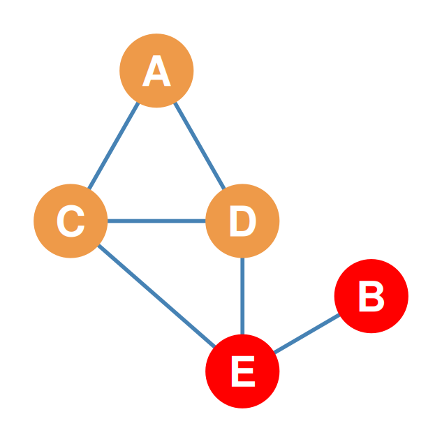
- No shared neighbors: the tie \(B\)–\(E\) (red) is all they have.
| A | B | C | D | E | |
|---|---|---|---|---|---|
| A | -- | 0.00 | 0.25 | 0.25 | 0.67 |
| B | 0.00 | -- | 0.33 | 0.33 | 0.00 |
| C | 0.25 | 0.33 | -- | 0.50 | 0.20 |
| D | 0.25 | 0.33 | 0.50 | -- | 0.20 |
| E | 0.67 | 0.00 | 0.20 | 0.20 | -- |
- \(\mathcal{N}(B) = \{E\}\) (\(k_B = 1\))
- \(\mathcal{N}(E) = \{B, C, D\}\) (\(k_E = 3\))
- Intersection: \(\mathcal{N}(B) \cap \mathcal{N}(E) = \varnothing\). Cardinality 0.
- Union: \(\{B, C, D, E\}\). Cardinality 4.
- Overlap: \[O_{BE} = \frac{0}{4} = 0.00\]
- \(B\) and \(E\) are tied but share nothing else — \(B\) is a pendant on \(E\), with no redundant contacts.