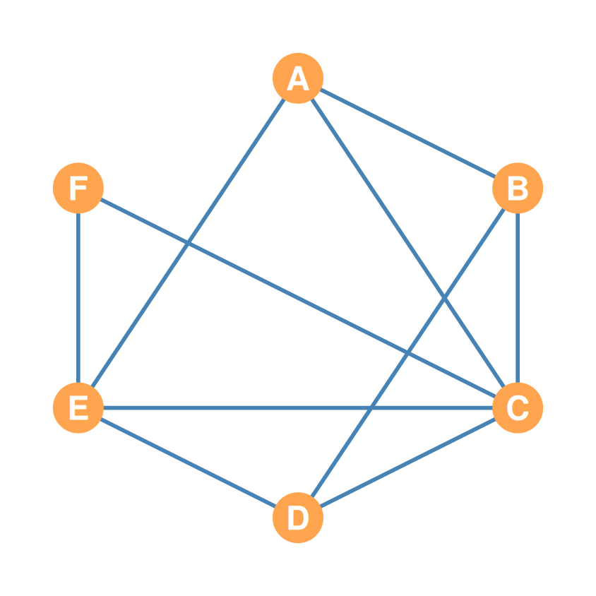
Matrix Algebra in Social Networks: Part II
Multiplication, Conformability, and Applications (Paths & Walks)
Transpose Multiplication (\(\mathbf{P} \times \mathbf{P}^T\)): Setup
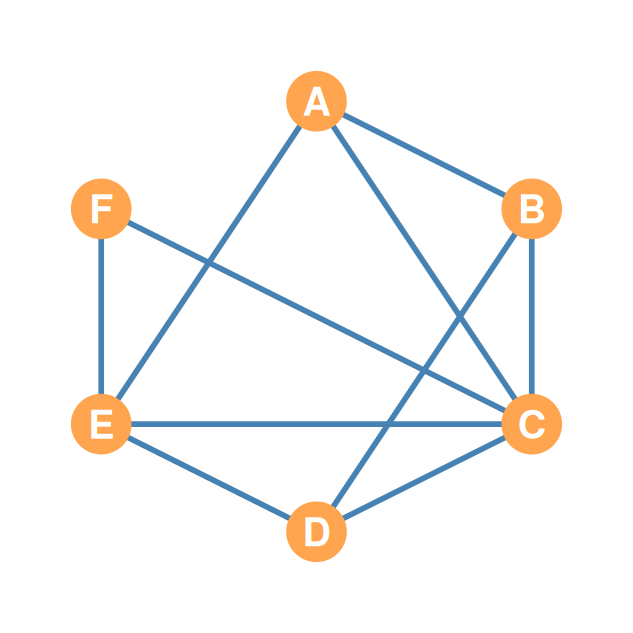
\(\mathbf{P}\) (the adjacency matrix)
| A | B | C | D | E | F | |
|---|---|---|---|---|---|---|
| A | 0 | 1 | 1 | 0 | 1 | 0 |
| B | 1 | 0 | 1 | 1 | 0 | 0 |
| C | 1 | 1 | 0 | 1 | 1 | 1 |
| D | 0 | 1 | 1 | 0 | 1 | 0 |
| E | 1 | 0 | 1 | 1 | 0 | 1 |
| F | 0 | 0 | 1 | 0 | 1 | 0 |
\(\mathbf{P}^T\) (columns of \(\mathbf{P}^T\) = rows of \(\mathbf{P}\))
| A | B | C | D | E | F | |
|---|---|---|---|---|---|---|
| A | 0 | 1 | 1 | 0 | 1 | 0 |
| B | 1 | 0 | 1 | 1 | 0 | 0 |
| C | 1 | 1 | 0 | 1 | 1 | 1 |
| D | 0 | 1 | 1 | 0 | 1 | 0 |
| E | 1 | 0 | 1 | 1 | 0 | 1 |
| F | 0 | 0 | 1 | 0 | 1 | 0 |
- Our \(6 \times 6\) “parties with” matrix \(\mathbf{P}\) is symmetric, so \(\mathbf{P}^T\) contains the same numbers — but read its entries by column: column \(j\) of \(\mathbf{P}^T\) is node \(j\)’s friendship row
- Multiplying \(\mathbf{P} \times \mathbf{P}^T\) therefore compares every node’s friendship row with every other node’s friendship row
Transpose Multiplication (\(\mathbf{P} \times \mathbf{P}^T\)): Diagonal Cells (Degrees)
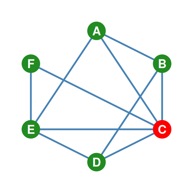
Row 3 of \(\mathbf{P}\) (C’s friendships)
| A | B | C | D | E | F | |
|---|---|---|---|---|---|---|
| A | 0 | 1 | 1 | 0 | 1 | 0 |
| B | 1 | 0 | 1 | 1 | 0 | 0 |
| C | 1 | 1 | 0 | 1 | 1 | 1 |
| D | 0 | 1 | 1 | 0 | 1 | 0 |
| E | 1 | 0 | 1 | 1 | 0 | 1 |
| F | 0 | 0 | 1 | 0 | 1 | 0 |
Column 3 of \(\mathbf{P}^T\) (= Row 3 of \(\mathbf{P}\))
| A | B | C | D | E | F | |
|---|---|---|---|---|---|---|
| A | 0 | 1 | 1 | 0 | 1 | 0 |
| B | 1 | 0 | 1 | 1 | 0 | 0 |
| C | 1 | 1 | 0 | 1 | 1 | 1 |
| D | 0 | 1 | 1 | 0 | 1 | 0 |
| E | 1 | 0 | 1 | 1 | 0 | 1 |
| F | 0 | 0 | 1 | 0 | 1 | 0 |
\[c_{33} = (\color{red}{1} \times \color{blue}{1}) + (\color{red}{1} \times \color{blue}{1}) + (\color{red}{0} \times \color{blue}{0}) + (\color{red}{1} \times \color{blue}{1}) + (\color{red}{1} \times \color{blue}{1}) + (\color{red}{1} \times \color{blue}{1}) = \mathbf{5}\]
- The diagonal recovers the degree sequence: \(c_{33} = 5\).
Transpose Multiplication: Another Diagonal Cell (\(p^T_{\text{E, E}}\))
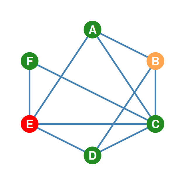
Row 5 of \(\mathbf{P}\) (E’s friendships)
| A | B | C | D | E | F | |
|---|---|---|---|---|---|---|
| A | 0 | 1 | 1 | 0 | 1 | 0 |
| B | 1 | 0 | 1 | 1 | 0 | 0 |
| C | 1 | 1 | 0 | 1 | 1 | 1 |
| D | 0 | 1 | 1 | 0 | 1 | 0 |
| E | 1 | 0 | 1 | 1 | 0 | 1 |
| F | 0 | 0 | 1 | 0 | 1 | 0 |
Column 5 of \(\mathbf{P}^T\) (= Row 5 of \(\mathbf{P}\))
| A | B | C | D | E | F | |
|---|---|---|---|---|---|---|
| A | 0 | 1 | 1 | 0 | 1 | 0 |
| B | 1 | 0 | 1 | 1 | 0 | 0 |
| C | 1 | 1 | 0 | 1 | 1 | 1 |
| D | 0 | 1 | 1 | 0 | 1 | 0 |
| E | 1 | 0 | 1 | 1 | 0 | 1 |
| F | 0 | 0 | 1 | 0 | 1 | 0 |
\[c_{55} = (\color{red}{1} \times \color{blue}{1}) + (\color{red}{0} \times \color{blue}{0}) + (\color{red}{1} \times \color{blue}{1}) + (\color{red}{1} \times \color{blue}{1}) + (\color{red}{0} \times \color{blue}{0}) + (\color{red}{1} \times \color{blue}{1}) = \mathbf{4}\]
- Node E has degree 4 (friends: A, C, D, F). The diagonal element \(c_{55} = 4\) is E’s degree.
Transpose Multiplication (\(\mathbf{P} \times \mathbf{P}^T\)): Off-Diagonal Cells (Common Neighbors)
Row 1 of \(\mathbf{P}\) (A’s friendships)
| A | B | C | D | E | F | |
|---|---|---|---|---|---|---|
| A | 0 | 1 | 1 | 0 | 1 | 0 |
| B | 1 | 0 | 1 | 1 | 0 | 0 |
| C | 1 | 1 | 0 | 1 | 1 | 1 |
| D | 0 | 1 | 1 | 0 | 1 | 0 |
| E | 1 | 0 | 1 | 1 | 0 | 1 |
| F | 0 | 0 | 1 | 0 | 1 | 0 |
Column 3 of \(\mathbf{P}^T\) (C’s friendships)
| A | B | C | D | E | F | |
|---|---|---|---|---|---|---|
| A | 0 | 1 | 1 | 0 | 1 | 0 |
| B | 1 | 0 | 1 | 1 | 0 | 0 |
| C | 1 | 1 | 0 | 1 | 1 | 1 |
| D | 0 | 1 | 1 | 0 | 1 | 0 |
| E | 1 | 0 | 1 | 1 | 0 | 1 |
| F | 0 | 0 | 1 | 0 | 1 | 0 |
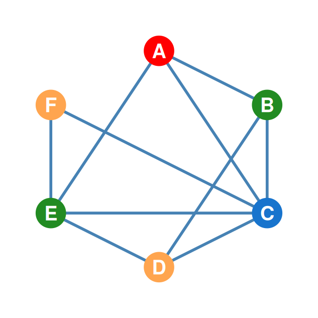
\[c_{\text{A, C}} = (\color{red}{0} \times \color{blue}{1}) + (\color{red}{1} \times \color{blue}{1}) + (\color{red}{1} \times \color{blue}{0}) + (\color{red}{0} \times \color{blue}{1}) + (\color{red}{1} \times \color{blue}{1}) + (\color{red}{0} \times \color{blue}{1}) = \mathbf{2}\]
- In the graph: red A, blue C, green shared friends. Each shared friend contributes \(\mathbf{1}\) (the bold pairs) — A and C share 2 common friends: B and E
Transpose Multiplication: Another Off-Diagonal Cell (\(p^T_{\text{B, E}}\))
Row 2 of \(\mathbf{P}\) (B’s friendships)
| A | B | C | D | E | F | |
|---|---|---|---|---|---|---|
| A | 0 | 1 | 1 | 0 | 1 | 0 |
| B | 1 | 0 | 1 | 1 | 0 | 0 |
| C | 1 | 1 | 0 | 1 | 1 | 1 |
| D | 0 | 1 | 1 | 0 | 1 | 0 |
| E | 1 | 0 | 1 | 1 | 0 | 1 |
| F | 0 | 0 | 1 | 0 | 1 | 0 |
Column 5 of \(\mathbf{P}^T\) (E’s friendships)
| A | B | C | D | E | F | |
|---|---|---|---|---|---|---|
| A | 0 | 1 | 1 | 0 | 1 | 0 |
| B | 1 | 0 | 1 | 1 | 0 | 0 |
| C | 1 | 1 | 0 | 1 | 1 | 1 |
| D | 0 | 1 | 1 | 0 | 1 | 0 |
| E | 1 | 0 | 1 | 1 | 0 | 1 |
| F | 0 | 0 | 1 | 0 | 1 | 0 |
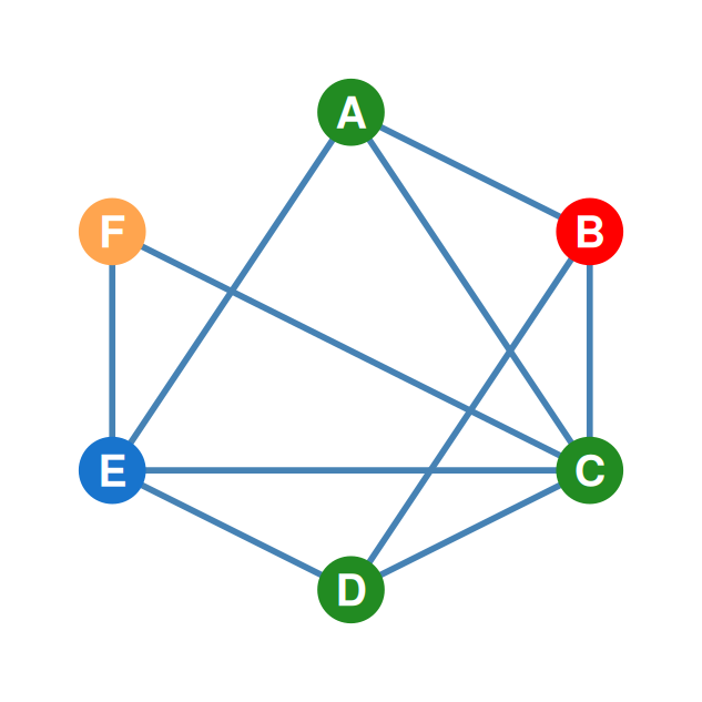
\[c_{\text{B, E}} = (\color{red}{1} \times \color{blue}{1}) + (\color{red}{1} \times \color{blue}{0}) + (\color{red}{1} \times \color{blue}{1}) + (\color{red}{1} \times \color{blue}{1}) + (\color{red}{0} \times \color{blue}{0}) + (\color{red}{0} \times \color{blue}{1}) = \mathbf{3}\]
- Red B and blue E share 3 common friends: A, C, D.
The Completed Product Matrix
| A | B | C | D | E | F | |
|---|---|---|---|---|---|---|
| A | 3 | 1 | 2 | 3 | 1 | 2 |
| B | 1 | 3 | 2 | 1 | 3 | 1 |
| C | 2 | 2 | 5 | 2 | 3 | 1 |
| D | 3 | 1 | 2 | 3 | 1 | 2 |
| E | 1 | 3 | 3 | 1 | 4 | 1 |
| F | 2 | 1 | 1 | 2 | 1 | 2 |
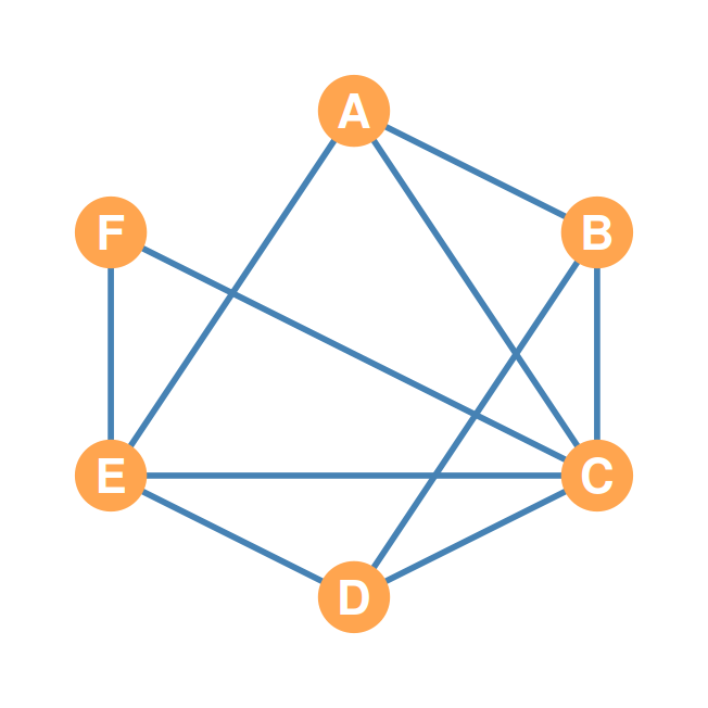
- Diagonal (shaded): degree of each node
- Off-diagonal: common friends between pairs
- Symmetric: friendship overlap is mutual
Directed Running Example: “Sends a Party Invitation To”
\(\mathbf{D}\) (the directed adjacency matrix)
| A | B | C | D | E | |
|---|---|---|---|---|---|
| A | 0 | 1 | 1 | 1 | 0 |
| B | 0 | 0 | 1 | 1 | 0 |
| C | 0 | 0 | 0 | 1 | 0 |
| D | 0 | 0 | 0 | 0 | 1 |
| E | 1 | 0 | 1 | 0 | 0 |
\(\mathbf{D}^T\) (rows of \(\mathbf{D}^T\) = columns of \(\mathbf{D}\))
| A | B | C | D | E | |
|---|---|---|---|---|---|
| A | 0 | 0 | 0 | 0 | 1 |
| B | 1 | 0 | 0 | 0 | 0 |
| C | 1 | 1 | 0 | 0 | 1 |
| D | 1 | 1 | 1 | 0 | 0 |
| E | 0 | 0 | 0 | 1 | 0 |
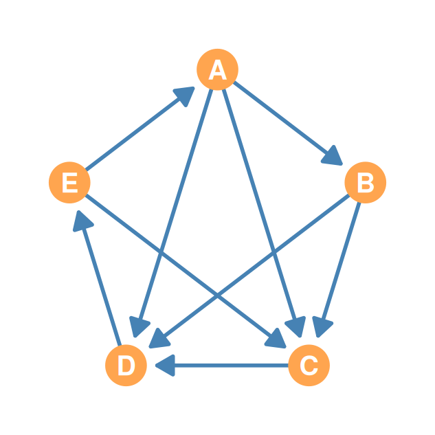
- New running example: five people (A–E); a tie \(i \rightarrow j\) means \(i\) invited \(j\)
- \(\mathbf{D}\) is not symmetric — choosing is not the same as being chosen — so \(\mathbf{D}^T\) is a genuinely different matrix
- Read \(\mathbf{D}\) by rows (out-ties: A invites B, C, D) and by columns (in-ties: C is invited by A, B, E)
Common Out-Neighbors (\(\mathbf{D} \times \mathbf{D}^T\)): Tracing the Diagonal Cell \((\mathbf{D}\mathbf{D}^T)_{\text{A, A}}\)
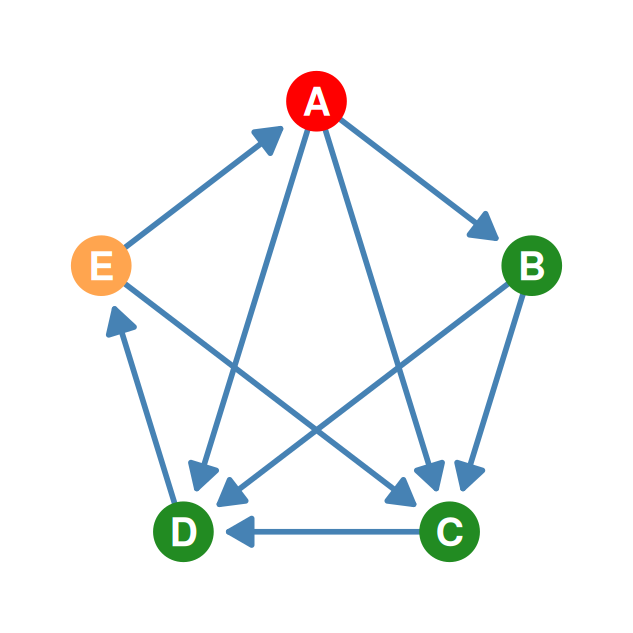
Row A of \(\mathbf{D}\) (A’s out-ties)
| A | B | C | D | E | |
|---|---|---|---|---|---|
| A | 0 | 1 | 1 | 1 | 0 |
| B | 0 | 0 | 1 | 1 | 0 |
| C | 0 | 0 | 0 | 1 | 0 |
| D | 0 | 0 | 0 | 0 | 1 |
| E | 1 | 0 | 1 | 0 | 0 |
Column A of \(\mathbf{D}^T\) (= Row A of \(\mathbf{D}\))
| A | B | C | D | E | |
|---|---|---|---|---|---|
| A | 0 | 0 | 0 | 0 | 1 |
| B | 1 | 0 | 0 | 0 | 0 |
| C | 1 | 1 | 0 | 0 | 1 |
| D | 1 | 1 | 1 | 0 | 0 |
| E | 0 | 0 | 0 | 1 | 0 |
\[c_{\text{A, A}} = (\color{red}{0} \times \color{blue}{0}) + (\color{red}{1} \times \color{blue}{1}) + (\color{red}{1} \times \color{blue}{1}) + (\color{red}{1} \times \color{blue}{1}) + (\color{red}{0} \times \color{blue}{0}) = \mathbf{3}\]
- A pairs with itself: every out-tie matches itself, so \(c_{\text{A, A}} = 3\) = A’s out-degree
Common Out-Neighbors (\(\mathbf{D} \times \mathbf{D}^T\)): Tracing Cell \((\mathbf{D}\mathbf{D}^T)_{\text{A, B}}\)
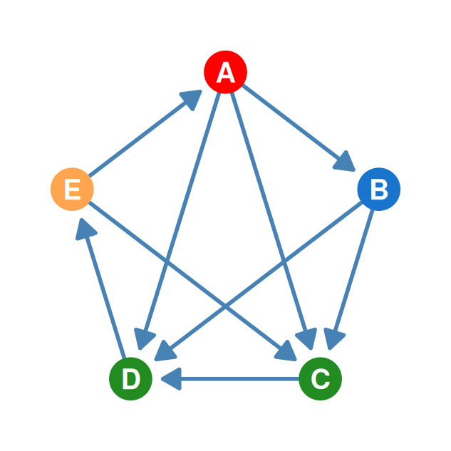
Row A of \(\mathbf{D}\) (A’s out-ties)
| A | B | C | D | E | |
|---|---|---|---|---|---|
| A | 0 | 1 | 1 | 1 | 0 |
| B | 0 | 0 | 1 | 1 | 0 |
| C | 0 | 0 | 0 | 1 | 0 |
| D | 0 | 0 | 0 | 0 | 1 |
| E | 1 | 0 | 1 | 0 | 0 |
Column B of \(\mathbf{D}^T\) (= Row B of \(\mathbf{D}\))
| A | B | C | D | E | |
|---|---|---|---|---|---|
| A | 0 | 0 | 0 | 0 | 1 |
| B | 1 | 0 | 0 | 0 | 0 |
| C | 1 | 1 | 0 | 0 | 1 |
| D | 1 | 1 | 1 | 0 | 0 |
| E | 0 | 0 | 0 | 1 | 0 |
\[c_{\text{A, B}} = (\color{red}{0} \times \color{blue}{0}) + (\color{red}{1} \times \color{blue}{0}) + (\color{red}{1} \times \color{blue}{1}) + (\color{red}{1} \times \color{blue}{1}) + (\color{red}{0} \times \color{blue}{0}) = \mathbf{2}\]
- Red A and blue B invited the same two people: C and D — 2 common out-neighbors
Common Out-Neighbors (\(\mathbf{D} \times \mathbf{D}^T\)): Tracing Cell \((\mathbf{D}\mathbf{D}^T)_{\text{C, D}}\)
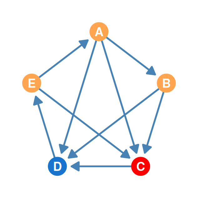
Row C of \(\mathbf{D}\) (C’s out-ties)
| A | B | C | D | E | |
|---|---|---|---|---|---|
| A | 0 | 1 | 1 | 1 | 0 |
| B | 0 | 0 | 1 | 1 | 0 |
| C | 0 | 0 | 0 | 1 | 0 |
| D | 0 | 0 | 0 | 0 | 1 |
| E | 1 | 0 | 1 | 0 | 0 |
Column D of \(\mathbf{D}^T\) (= Row D of \(\mathbf{D}\))
| A | B | C | D | E | |
|---|---|---|---|---|---|
| A | 0 | 0 | 0 | 0 | 1 |
| B | 1 | 0 | 0 | 0 | 0 |
| C | 1 | 1 | 0 | 0 | 1 |
| D | 1 | 1 | 1 | 0 | 0 |
| E | 0 | 0 | 0 | 1 | 0 |
\[c_{\text{C, D}} = (\color{red}{0} \times \color{blue}{0}) + (\color{red}{0} \times \color{blue}{0}) + (\color{red}{0} \times \color{blue}{0}) + (\color{red}{1} \times \color{blue}{0}) + (\color{red}{0} \times \color{blue}{1}) = \mathbf{0}\]
- Red C invites only D; blue D invites only E — nothing in green: 0 common out-neighbors
The Completed \(\mathbf{D} \times \mathbf{D}^T\) Matrix
| A | B | C | D | E | |
|---|---|---|---|---|---|
| A | 3 | 2 | 1 | 0 | 1 |
| B | 2 | 2 | 1 | 0 | 1 |
| C | 1 | 1 | 1 | 0 | 0 |
| D | 0 | 0 | 0 | 1 | 0 |
| E | 1 | 1 | 0 | 0 | 2 |
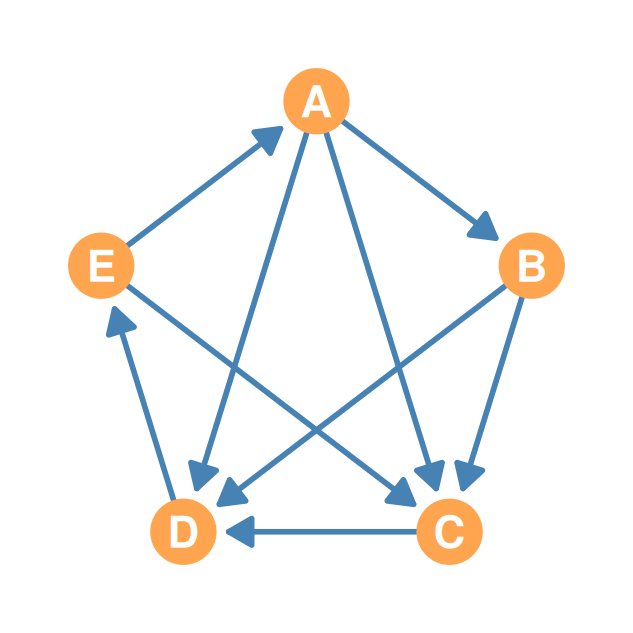
- Diagonal (shaded): the out-degrees
- Off-diagonal: how many people two nodes both invited
- Symmetric — even though \(\mathbf{D}\) itself is not
Common In-Neighbors (\(\mathbf{D}^T \times \mathbf{D}\)): Tracing the Diagonal Cell \((\mathbf{D}^T\mathbf{D})_{\text{C, C}}\)
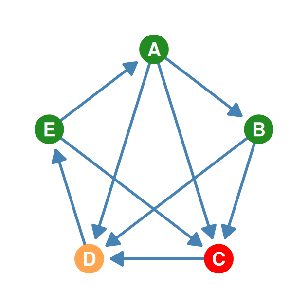
Row C of \(\mathbf{D}^T\) (who invited C)
| A | B | C | D | E | |
|---|---|---|---|---|---|
| A | 0 | 0 | 0 | 0 | 1 |
| B | 1 | 0 | 0 | 0 | 0 |
| C | 1 | 1 | 0 | 0 | 1 |
| D | 1 | 1 | 1 | 0 | 0 |
| E | 0 | 0 | 0 | 1 | 0 |
Column C of \(\mathbf{D}\) (who invited C)
| A | B | C | D | E | |
|---|---|---|---|---|---|
| A | 0 | 1 | 1 | 1 | 0 |
| B | 0 | 0 | 1 | 1 | 0 |
| C | 0 | 0 | 0 | 1 | 0 |
| D | 0 | 0 | 0 | 0 | 1 |
| E | 1 | 0 | 1 | 0 | 0 |
\[c_{\text{C, C}} = (\color{red}{1} \times \color{blue}{1}) + (\color{red}{1} \times \color{blue}{1}) + (\color{red}{0} \times \color{blue}{0}) + (\color{red}{0} \times \color{blue}{0}) + (\color{red}{1} \times \color{blue}{1}) = \mathbf{3}\]
- C pairs with itself: every in-tie matches itself, so \(c_{\text{C, C}} = 3\) = C’s in-degree (A, B, and E invited C)
Common In-Neighbors (\(\mathbf{D}^T \times \mathbf{D}\)): Tracing Cell \((\mathbf{D}^T\mathbf{D})_{\text{C, D}}\)
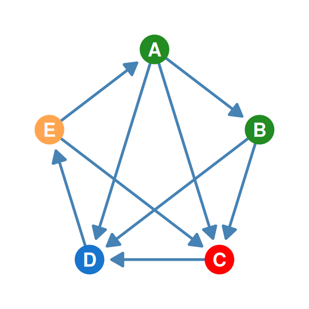
Row C of \(\mathbf{D}^T\) (who invited C)
| A | B | C | D | E | |
|---|---|---|---|---|---|
| A | 0 | 0 | 0 | 0 | 1 |
| B | 1 | 0 | 0 | 0 | 0 |
| C | 1 | 1 | 0 | 0 | 1 |
| D | 1 | 1 | 1 | 0 | 0 |
| E | 0 | 0 | 0 | 1 | 0 |
Column D of \(\mathbf{D}\) (who invited D)
| A | B | C | D | E | |
|---|---|---|---|---|---|
| A | 0 | 1 | 1 | 1 | 0 |
| B | 0 | 0 | 1 | 1 | 0 |
| C | 0 | 0 | 0 | 1 | 0 |
| D | 0 | 0 | 0 | 0 | 1 |
| E | 1 | 0 | 1 | 0 | 0 |
\[c_{\text{C, D}} = (\color{red}{1} \times \color{blue}{1}) + (\color{red}{1} \times \color{blue}{1}) + (\color{red}{0} \times \color{blue}{1}) + (\color{red}{0} \times \color{blue}{0}) + (\color{red}{1} \times \color{blue}{0}) = \mathbf{2}\]
- Rows of \(\mathbf{D}^T\) are \(\mathbf{D}\)’s columns: in-tie lists. Red C and blue D were invited by the same two people: A and B — 2 common in-neighbors
Common In-Neighbors (\(\mathbf{D}^T \times \mathbf{D}\)): Tracing Cell \((\mathbf{D}^T\mathbf{D})_{\text{A, B}}\)
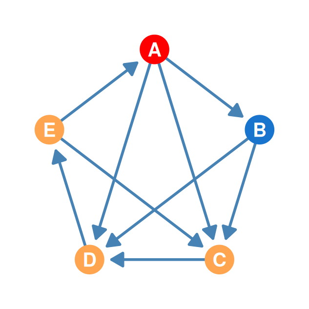
Row A of \(\mathbf{D}^T\) (who invited A)
| A | B | C | D | E | |
|---|---|---|---|---|---|
| A | 0 | 0 | 0 | 0 | 1 |
| B | 1 | 0 | 0 | 0 | 0 |
| C | 1 | 1 | 0 | 0 | 1 |
| D | 1 | 1 | 1 | 0 | 0 |
| E | 0 | 0 | 0 | 1 | 0 |
Column B of \(\mathbf{D}\) (who invited B)
| A | B | C | D | E | |
|---|---|---|---|---|---|
| A | 0 | 1 | 1 | 1 | 0 |
| B | 0 | 0 | 1 | 1 | 0 |
| C | 0 | 0 | 0 | 1 | 0 |
| D | 0 | 0 | 0 | 0 | 1 |
| E | 1 | 0 | 1 | 0 | 0 |
\[c_{\text{A, B}} = (\color{red}{0} \times \color{blue}{1}) + (\color{red}{0} \times \color{blue}{0}) + (\color{red}{0} \times \color{blue}{0}) + (\color{red}{0} \times \color{blue}{0}) + (\color{red}{1} \times \color{blue}{0}) = \mathbf{0}\]
- Only E invites A and only A invites B — nobody invites both: 0 common in-neighbors
The Completed \(\mathbf{D}^T \times \mathbf{D}\) Matrix
| A | B | C | D | E | |
|---|---|---|---|---|---|
| A | 1 | 0 | 1 | 0 | 0 |
| B | 0 | 1 | 1 | 1 | 0 |
| C | 1 | 1 | 3 | 2 | 0 |
| D | 0 | 1 | 2 | 3 | 0 |
| E | 0 | 0 | 0 | 0 | 1 |
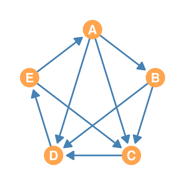
- Diagonal (shaded): the in-degrees
- Off-diagonal: how many senders two nodes share
- The payoff: A and B share 2 out-neighbors but 0 in-neighbors; C and D are the mirror image
Walks of Length 2 (\(\mathbf{P}^2\)): Tracing Cell \(p^2_{\text{A, C}}\)
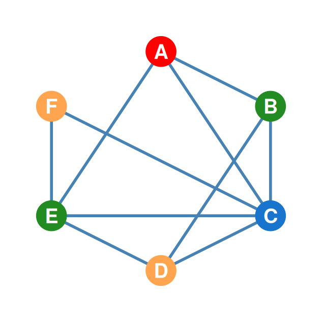
Row 1 of \(\mathbf{P}\) (A’s friendships)
| A | B | C | D | E | F | |
|---|---|---|---|---|---|---|
| A | 0 | 1 | 1 | 0 | 1 | 0 |
| B | 1 | 0 | 1 | 1 | 0 | 0 |
| C | 1 | 1 | 0 | 1 | 1 | 1 |
| D | 0 | 1 | 1 | 0 | 1 | 0 |
| E | 1 | 0 | 1 | 1 | 0 | 1 |
| F | 0 | 0 | 1 | 0 | 1 | 0 |
Column 3 of \(\mathbf{P}\) (C’s friendships)
| A | B | C | D | E | F | |
|---|---|---|---|---|---|---|
| A | 0 | 1 | 1 | 0 | 1 | 0 |
| B | 1 | 0 | 1 | 1 | 0 | 0 |
| C | 1 | 1 | 0 | 1 | 1 | 1 |
| D | 0 | 1 | 1 | 0 | 1 | 0 |
| E | 1 | 0 | 1 | 1 | 0 | 1 |
| F | 0 | 0 | 1 | 0 | 1 | 0 |
\[p^2_{\text{A, C}} = (\color{red}{0} \times \color{blue}{1}) + (\color{red}{1} \times \color{blue}{1}) + (\color{red}{1} \times \color{blue}{0}) + (\color{red}{0} \times \color{blue}{1}) + (\color{red}{1} \times \color{blue}{1}) + (\color{red}{0} \times \color{blue}{1}) = \mathbf{2}\]
- In the graph: red A, blue C, green shared friends. The two walks are \(A \rightarrow \mathbf{B} \rightarrow C\) and \(A \rightarrow \mathbf{E} \rightarrow C\) — exactly the 2 common friends we found for \(c_{\text{A, C}}\) earlier!
Walks of Length 2 (\(\mathbf{P}^2\)): Tracing Diagonal Cell \(p^2_{\text{C, C}}\)
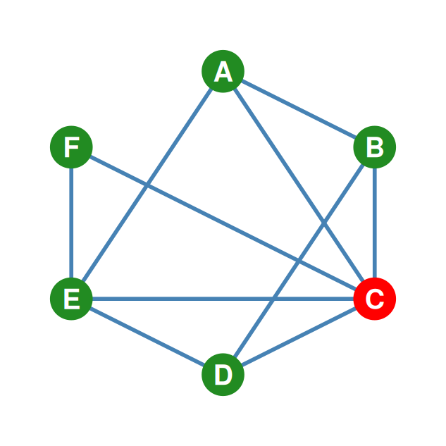
Row 3 of \(\mathbf{P}\) (C’s friendships)
| A | B | C | D | E | F | |
|---|---|---|---|---|---|---|
| A | 0 | 1 | 1 | 0 | 1 | 0 |
| B | 1 | 0 | 1 | 1 | 0 | 0 |
| C | 1 | 1 | 0 | 1 | 1 | 1 |
| D | 0 | 1 | 1 | 0 | 1 | 0 |
| E | 1 | 0 | 1 | 1 | 0 | 1 |
| F | 0 | 0 | 1 | 0 | 1 | 0 |
Column 3 of \(\mathbf{P}\) (also C’s friendships)
| A | B | C | D | E | F | |
|---|---|---|---|---|---|---|
| A | 0 | 1 | 1 | 0 | 1 | 0 |
| B | 1 | 0 | 1 | 1 | 0 | 0 |
| C | 1 | 1 | 0 | 1 | 1 | 1 |
| D | 0 | 1 | 1 | 0 | 1 | 0 |
| E | 1 | 0 | 1 | 1 | 0 | 1 |
| F | 0 | 0 | 1 | 0 | 1 | 0 |
\[p^2_{\text{C, C}} = (\color{red}{1} \times \color{blue}{1}) + (\color{red}{1} \times \color{blue}{1}) + (\color{red}{0} \times \color{blue}{0}) + (\color{red}{1} \times \color{blue}{1}) + (\color{red}{1} \times \color{blue}{1}) + (\color{red}{1} \times \color{blue}{1}) = \mathbf{5}\]
- Walks from C back to C are round trips to each friend (\(C \rightarrow A \rightarrow C\), etc.) — the diagonal of \(\mathbf{P}^2\) recovers the degrees, same as \(\mathbf{P} \times \mathbf{P}^T\)!
Walks of Length 3 (\(\mathbf{P}^3\)): Tracing Cell \(p^3_{\text{A, D}}\)
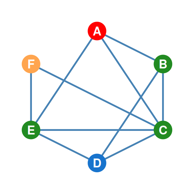
Row 1 of \(\mathbf{P}^2\) (A’s length-2 walks)
| A | B | C | D | E | F | |
|---|---|---|---|---|---|---|
| A | 3 | 1 | 2 | 3 | 1 | 2 |
| B | 1 | 3 | 2 | 1 | 3 | 1 |
| C | 2 | 2 | 5 | 2 | 3 | 1 |
| D | 3 | 1 | 2 | 3 | 1 | 2 |
| E | 1 | 3 | 3 | 1 | 4 | 1 |
| F | 2 | 1 | 1 | 2 | 1 | 2 |
Column 4 of \(\mathbf{P}\) (D’s friendships)
| A | B | C | D | E | F | |
|---|---|---|---|---|---|---|
| A | 0 | 1 | 1 | 0 | 1 | 0 |
| B | 1 | 0 | 1 | 1 | 0 | 0 |
| C | 1 | 1 | 0 | 1 | 1 | 1 |
| D | 0 | 1 | 1 | 0 | 1 | 0 |
| E | 1 | 0 | 1 | 1 | 0 | 1 |
| F | 0 | 0 | 1 | 0 | 1 | 0 |
\[p^3_{\text{A, D}} = (\color{red}{3} \times \color{blue}{0}) + (\color{red}{1} \times \color{blue}{1}) + (\color{red}{2} \times \color{blue}{1}) + (\color{red}{3} \times \color{blue}{0}) + (\color{red}{1} \times \color{blue}{1}) + (\color{red}{2} \times \color{blue}{0}) = \mathbf{4}\]
- A and D are not adjacent but share friends B, C, E — and all 4 walks stay in that cluster: \(A \rightarrow B \rightarrow C \rightarrow D\), \(A \rightarrow C \rightarrow B \rightarrow D\), \(A \rightarrow C \rightarrow E \rightarrow D\), \(A \rightarrow E \rightarrow C \rightarrow D\).
Walks of Length 3 (\(\mathbf{P}^3\)): An Adjacent Pair, \(p^3_{\text{A, C}}\)
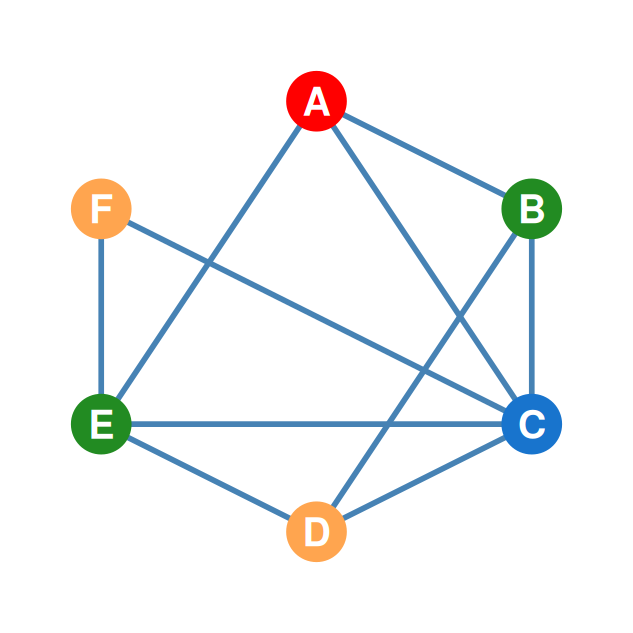
Row 1 of \(\mathbf{P}^2\) (A’s length-2 walks)
| A | B | C | D | E | F | |
|---|---|---|---|---|---|---|
| A | 3 | 1 | 2 | 3 | 1 | 2 |
| B | 1 | 3 | 2 | 1 | 3 | 1 |
| C | 2 | 2 | 5 | 2 | 3 | 1 |
| D | 3 | 1 | 2 | 3 | 1 | 2 |
| E | 1 | 3 | 3 | 1 | 4 | 1 |
| F | 2 | 1 | 1 | 2 | 1 | 2 |
Column 3 of \(\mathbf{P}\) (C’s friendships)
| A | B | C | D | E | F | |
|---|---|---|---|---|---|---|
| A | 0 | 1 | 1 | 0 | 1 | 0 |
| B | 1 | 0 | 1 | 1 | 0 | 0 |
| C | 1 | 1 | 0 | 1 | 1 | 1 |
| D | 0 | 1 | 1 | 0 | 1 | 0 |
| E | 1 | 0 | 1 | 1 | 0 | 1 |
| F | 0 | 0 | 1 | 0 | 1 | 0 |
\[p^3_{\text{A, C}} = (\color{red}{3} \times \color{blue}{1}) + (\color{red}{1} \times \color{blue}{1}) + (\color{red}{2} \times \color{blue}{0}) + (\color{red}{3} \times \color{blue}{1}) + (\color{red}{1} \times \color{blue}{1}) + (\color{red}{2} \times \color{blue}{1}) = \mathbf{10}\]
- A and C are adjacent, so the 10 walks include backtracking like \(A \rightarrow B \rightarrow A \rightarrow C\) — off-diagonal \(\mathbf{P}^3\) counts every walk, not just sensible paths.
Walks of Length 3 (\(\mathbf{P}^3\)): Tracing Diagonal Cell \(p^3_{\text{C, C}}\)
Row 3 of \(\mathbf{P}^2\) (C’s length-2 walks)
| A | B | C | D | E | F | |
|---|---|---|---|---|---|---|
| A | 3 | 1 | 2 | 3 | 1 | 2 |
| B | 1 | 3 | 2 | 1 | 3 | 1 |
| C | 2 | 2 | 5 | 2 | 3 | 1 |
| D | 3 | 1 | 2 | 3 | 1 | 2 |
| E | 1 | 3 | 3 | 1 | 4 | 1 |
| F | 2 | 1 | 1 | 2 | 1 | 2 |
Column 3 of \(\mathbf{P}\) (C’s friendships)
| A | B | C | D | E | F | |
|---|---|---|---|---|---|---|
| A | 0 | 1 | 1 | 0 | 1 | 0 |
| B | 1 | 0 | 1 | 1 | 0 | 0 |
| C | 1 | 1 | 0 | 1 | 1 | 1 |
| D | 0 | 1 | 1 | 0 | 1 | 0 |
| E | 1 | 0 | 1 | 1 | 0 | 1 |
| F | 0 | 0 | 1 | 0 | 1 | 0 |
\[p^3_{\text{C, C}} = (\color{red}{2} \times \color{blue}{1}) + (\color{red}{2} \times \color{blue}{1}) + (\color{red}{5} \times \color{blue}{0}) + (\color{red}{2} \times \color{blue}{1}) + (\color{red}{3} \times \color{blue}{1}) + (\color{red}{1} \times \color{blue}{1}) = \mathbf{10}\]
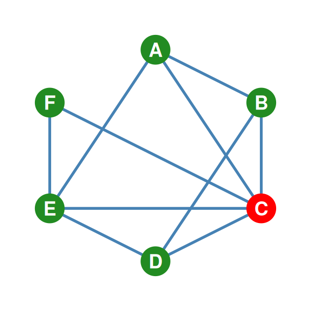
- Node C belongs to 5 triangles: \(\text{Triangles}(C) = p^3_{\text{C, C}}/2 = 10/2\) — each triangle counts twice (once per direction).
Summary: Matrix Multiplication in Networks
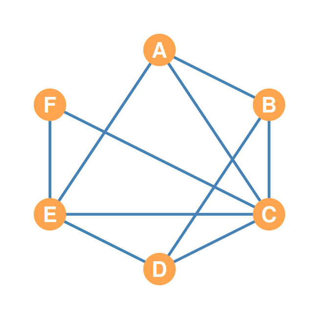
- The running example: six friends and their “parties with” ties
One worked example, five operations:
| Operation | What_it_reveals |
|---|---|
| P + G | Multiplex ties: connected in both networks |
| Pᵀ (transpose) | Reversed tie direction; feeds the dyad census |
| P × Pᵀ | Common neighbors (off-diagonal); degrees (diagonal) |
| P² = P × P | Number of walks of length 2 (= common neighbors) |
| P³ = P² × P | Walks of length 3; diagonal ÷ 2 = triangles |
| D × Dᵀ, Dᵀ × D (directed) | Common out-neighbors vs. common in-neighbors; diagonals = out- / in-degrees |