Matrix Algebra in Social Networks: Part I

Basic Operations, Transpose, and the Dyad Census

Part 1: Basic Operations & Network Overlap

Combining Social Relations

  • In social network analysis, we often record multiple types of relationships for the same set of nodes (e.g., Parties With vs. Plays Games With).
  • How do we combine, subtract, or intersect these overlapping structures?
  • We use Basic Matrix Operations performed cell-by-cell on adjacency matrices of the same dimensions:
    1. Matrix Addition (\(\mathbf{P} + \mathbf{G}\)): Measures overall relationship volume (uniplex vs. multiplex).
    2. Subtracting from a Matrix (\(\mathbf{1} - \mathbf{P}\)): Flips ties to find the graph complement (Does Not Party With).
    3. Hadamard Product (\(\mathbf{P} \circ \mathbf{G}\)): Extracts multiplex overlap (Parties and Plays Games With).

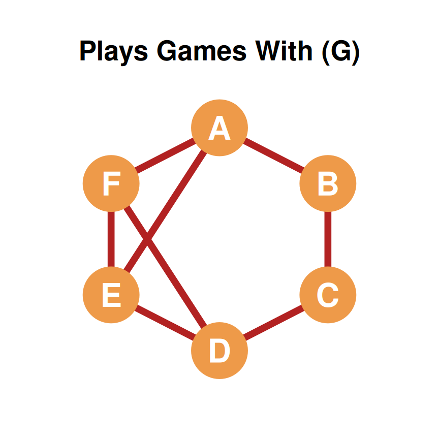
Meet the Networks: Parties With and Plays Games With

  • To make things concrete, consider a group of six people, labeled A through F.
  • For this same group we have recorded two separate social relationships:
    • Parties With: a tie joins two people if they have partied together.
    • Plays Games With: a tie joins two people if they play games together.
  • The same six people appear in both networks, so the two structures are directly comparable — and combinable.
  • We will refer to these two networks (and their matrices) as \(\mathbf{P}\) and \(\mathbf{G}\).

The Two Networks as Graphs

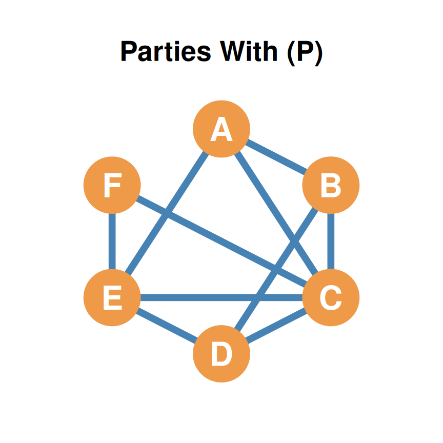
Adjacency Matrix: Parties With (\(\mathbf{P}\))

Parties With (\(\mathbf{P}\))

A B C D E F
A -- 1 1 0 1 0
B 1 -- 1 1 0 0
C 1 1 -- 1 1 1
D 0 1 1 -- 1 0
E 1 0 1 1 -- 1
F 0 0 1 0 1 --
  • The matrix is symmetric: ties are undirected.
  • Diagonal is always zero (no self-ties).
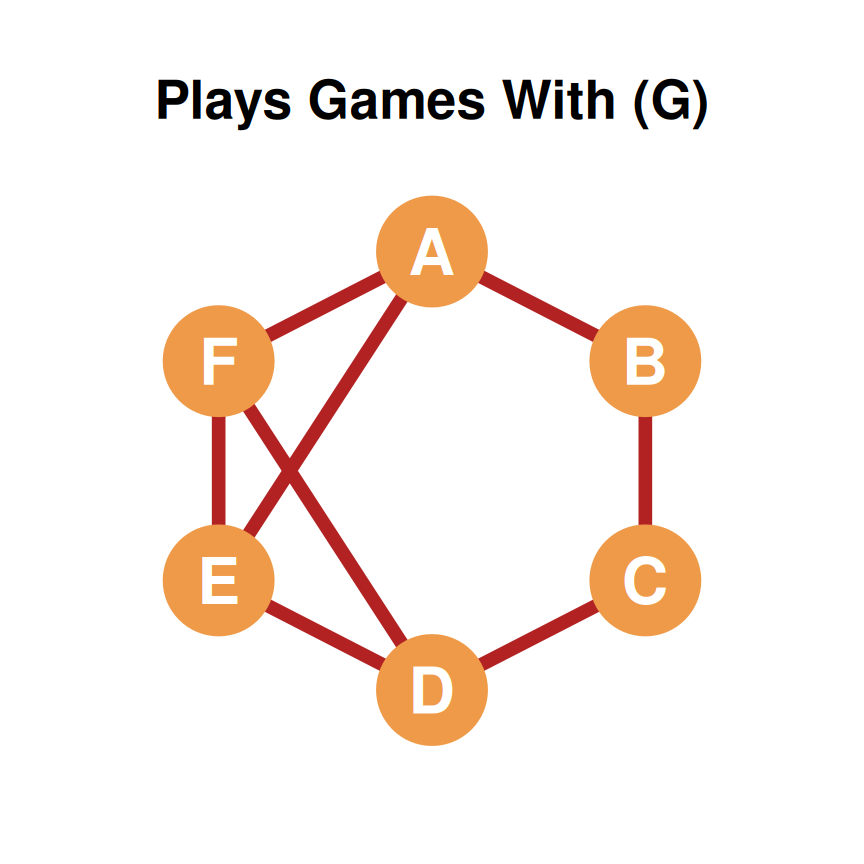
Adjacency Matrix: Plays Games With (\(\mathbf{G}\))

Plays Games With (\(\mathbf{G}\))

A B C D E F
A -- 1 0 0 1 1
B 1 -- 1 0 0 0
C 0 1 -- 1 0 0
D 0 0 1 -- 1 1
E 1 0 0 1 -- 1
F 1 0 0 1 1 --
  • Same nodes as \(\mathbf{P}\), but a different relation.
  • Same dimensions, so \(\mathbf{P}\) and \(\mathbf{G}\) can be combined cell-by-cell.
Step-by-Step Addition (\(\mathbf{P} + \mathbf{G}\)): Setup

  • Addition (\(s_{ij} = p_{ij} + g_{ij}\)) adds corresponding cells of each matrix.
  • Let’s trace how the resulting sum matrix is constructed from the first two:
    • \(s_{\text{A, B}} = p_{\text{A, B}} + g_{\text{A, B}} = 1 + 1 = \mathbf{2}\) (Multiplex)
    • \(s_{\text{A, C}} = p_{\text{A, C}} + g_{\text{A, C}} = 1 + 0 = \mathbf{1}\) (Uniplex)

\[\mathbf{P} + \mathbf{G} = \begin{pmatrix} 0 & 1 & 1 & 0 & 1 & 0 \\ 1 & 0 & 1 & 1 & 0 & 0 \\ 1 & 1 & 0 & 1 & 1 & 1 \\ 0 & 1 & 1 & 0 & 1 & 0 \\ 1 & 0 & 1 & 1 & 0 & 1 \\ 0 & 0 & 1 & 0 & 1 & 0 \end{pmatrix} + \begin{pmatrix} 0 & 1 & 0 & 0 & 1 & 1 \\ 1 & 0 & 1 & 0 & 0 & 0 \\ 0 & 1 & 0 & 1 & 0 & 0 \\ 0 & 0 & 1 & 0 & 1 & 1 \\ 1 & 0 & 0 & 1 & 0 & 1 \\ 1 & 0 & 0 & 1 & 1 & 0 \end{pmatrix}\]

Step-by-Step Addition (\(\mathbf{P} + \mathbf{G}\)): Calculation

  • We add the entries cell-by-cell:

\[\mathbf{P} + \mathbf{G} = \begin{pmatrix} 0+0 & 1+1 & 1+0 & 0+0 & 1+1 & 0+1 \\ 1+1 & 0+0 & 1+1 & 1+0 & 0+0 & 0+0 \\ 1+0 & 1+1 & 0+0 & 1+1 & 1+0 & 1+0 \\ 0+0 & 1+0 & 1+1 & 0+0 & 1+1 & 0+1 \\ 1+1 & 0+0 & 1+0 & 1+1 & 0+0 & 1+1 \\ 0+1 & 0+0 & 1+0 & 0+1 & 1+1 & 0+0 \end{pmatrix}\]

Step-by-Step Addition (\(\mathbf{P} + \mathbf{G}\)): Result

\[\mathbf{P} + \mathbf{G} = \begin{pmatrix} 0 & \mathbf{2} & 1 & 0 & \mathbf{2} & 1 \\ \mathbf{2} & 0 & \mathbf{2} & 1 & 0 & 0 \\ 1 & \mathbf{2} & 0 & \mathbf{2} & 1 & 1 \\ 0 & 1 & \mathbf{2} & 0 & \mathbf{2} & 1 \\ \mathbf{2} & 0 & 1 & \mathbf{2} & 0 & \mathbf{2} \\ 1 & 0 & 1 & 1 & \mathbf{2} & 0 \end{pmatrix}\]

  • Sociological Interpretation of the cell-by-cell sum:
    • Value 2 represents a multiplex tie (connected by both relationships).
    • Value 1 represents a uniplex tie (connected by exactly one relationship).
    • Value 0 represents no relationship.

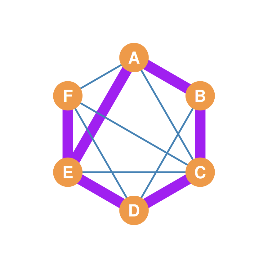
Visualizing Matrix Addition (\(\mathbf{P} + \mathbf{G}\))

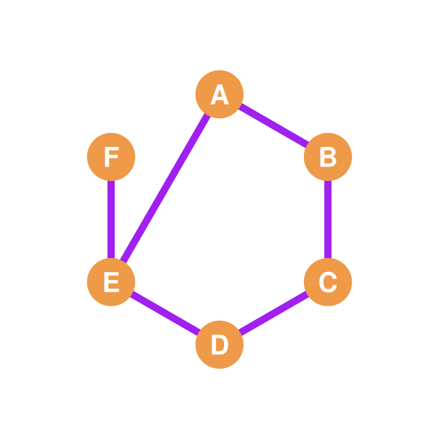
Parties or Plays Games With or Both

A B C D E F
A -- 2 1 0 2 1
B 2 -- 2 1 0 0
C 1 2 -- 2 1 1
D 0 1 2 -- 2 1
E 2 0 1 2 -- 2
F 1 0 1 1 2 --
  • 1 (Blue) = Uniplex bond.
  • 2 (Purple) = Multiplex bond.

Subtracting a Number From a Matrix (\(\mathbf{1} - \mathbf{P}\)): Setup

  • We can subtract an adjacency matrix from 1 (excluding the diagonal) to find the graph complement.
  • Subtracting from 1 flips 1s into 0s and 0s into 1s:
    • \(c_{ij} = 1 - p_{ij}\)

\[\mathbf{1} - \mathbf{P} = 1 - \begin{pmatrix} - & 1 & 1 & 0 & 1 & 0 \\ 1 & - & 1 & 1 & 0 & 0 \\ 1 & 1 & - & 1 & 1 & 1 \\ 0 & 1 & 1 & - & 1 & 0 \\ 1 & 0 & 1 & 1 & - & 1 \\ 0 & 0 & 1 & 0 & 1 & - \end{pmatrix}\]

Subtracting a Number From a Matrix (\(\mathbf{1} - \mathbf{P}\)): Calculation

  • Subtracting each cell from 1 yields:

\[\mathbf{1} - \mathbf{P} = \begin{pmatrix} - & 1-1 & 1-1 & 1-0 & 1-1 & 1-0 \\ 1-1 & - & 1-1 & 1-1 & 1-0 & 1-0 \\ 1-1 & 1-1 & - & 1-1 & 1-1 & 1-1 \\ 1-0 & 1-1 & 1-1 & - & 1-1 & 1-0 \\ 1-1 & 1-0 & 1-1 & 1-1 & - & 1-1 \\ 1-0 & 1-0 & 1-1 & 1-0 & 1-1 & - \end{pmatrix}\]

Subtracting a Number From a Matrix (\(\mathbf{1} - \mathbf{P}\)): Result

  • Flipping every off-diagonal cell yields the complement matrix:

\[\mathbf{1} - \mathbf{P} = \begin{pmatrix} - & 0 & 0 & 1 & 0 & 1 \\ 0 & - & 0 & 0 & 1 & 1 \\ 0 & 0 & - & 0 & 0 & 0 \\ 1 & 0 & 0 & - & 0 & 1 \\ 0 & 1 & 0 & 0 & - & 0 \\ 1 & 1 & 0 & 1 & 0 & - \end{pmatrix}\]

  • Sociological Meaning:
    • The resulting matrix records the absence of the original relationship.
    • The graph corresponding to this matrix is called the complement of the original graph (Does Not Party With).

Visualizing Graph Complement (\(\mathbf{1} - \mathbf{P}\))

Does Not Party With

A B C D E F
A -- 0 0 1 0 1
B 0 -- 0 0 1 1
C 0 0 -- 0 0 0
D 1 0 0 -- 0 1
E 0 1 0 0 -- 0
F 1 1 0 1 0 --
  • Holds \(1\)s where there was no original tie.
  • Diagonal remains blocked.

Step-by-Step Hadamard Product (\(\mathbf{P} \circ \mathbf{G}\)): Setup

  • Hadamard / Element-Wise Product (\(c_{ij} = p_{ij} \times g_{ij}\)) represents relational intersection:
  • Let’s trace how the multiplex intersection emerges from the product of the first two matrices:
    • \(c_{\text{A, B}} = p_{\text{A, B}} \times g_{\text{A, B}} = 1 \times 1 = \mathbf{1}\) (Both active)
    • \(c_{\text{A, C}} = p_{\text{A, C}} \times g_{\text{A, C}} = 1 \times 0 = \mathbf{0}\) (Only one active)

\[\mathbf{P} \circ \mathbf{G} = \begin{pmatrix} 0 & 1 & 1 & 0 & 1 & 0 \\ 1 & 0 & 1 & 1 & 0 & 0 \\ 1 & 1 & 0 & 1 & 1 & 1 \\ 0 & 1 & 1 & 0 & 1 & 0 \\ 1 & 0 & 1 & 1 & 0 & 1 \\ 0 & 0 & 1 & 0 & 1 & 0 \end{pmatrix} \circ \begin{pmatrix} 0 & 1 & 0 & 0 & 1 & 1 \\ 1 & 0 & 1 & 0 & 0 & 0 \\ 0 & 1 & 0 & 1 & 0 & 0 \\ 0 & 0 & 1 & 0 & 1 & 1 \\ 1 & 0 & 0 & 1 & 0 & 1 \\ 1 & 0 & 0 & 1 & 1 & 0 \end{pmatrix}\]

Step-by-Step Hadamard Product (\(\mathbf{P} \circ \mathbf{G}\)): Calculation

  • Multiplying corresponding entries cell-by-cell yields:

\[\mathbf{P} \circ \mathbf{G} = \begin{pmatrix} 0\times0 & 1\times1 & 1\times0 & 0\times0 & 1\times1 & 0\times1 \\ 1\times1 & 0\times0 & 1\times1 & 1\times0 & 0\times0 & 0\times0 \\ 1\times0 & 1\times1 & 0\times0 & 1\times1 & 1\times0 & 1\times0 \\ 0\times0 & 1\times0 & 1\times1 & 0\times0 & 1\times1 & 0\times1 \\ 1\times1 & 0\times0 & 1\times0 & 1\times1 & 0\times0 & 1\times1 \\ 0\times1 & 0\times0 & 1\times0 & 0\times1 & 1\times1 & 0\times0 \end{pmatrix}\]

Step-by-Step Hadamard Product (\(\mathbf{P} \circ \mathbf{G}\)): Result

  • Cell-by-cell multiplication yields the intersection matrix:

\[\mathbf{P} \circ \mathbf{G} = \begin{pmatrix} 0 & \mathbf{1} & 0 & 0 & \mathbf{1} & 0 \\ \mathbf{1} & 0 & \mathbf{1} & 0 & 0 & 0 \\ 0 & \mathbf{1} & 0 & \mathbf{1} & 0 & 0 \\ 0 & 0 & \mathbf{1} & 0 & \mathbf{1} & 0 \\ \mathbf{1} & 0 & 0 & \mathbf{1} & 0 & \mathbf{1} \\ 0 & 0 & 0 & 0 & \mathbf{1} & 0 \end{pmatrix}\]

  • Sociological Meaning:
    • Cell value is 1 only if both \(p_{ij} = 1\) and \(g_{ij} = 1\).
    • It extracts multiplex ties (the overlap/intersection) and erases all uniplex ties.

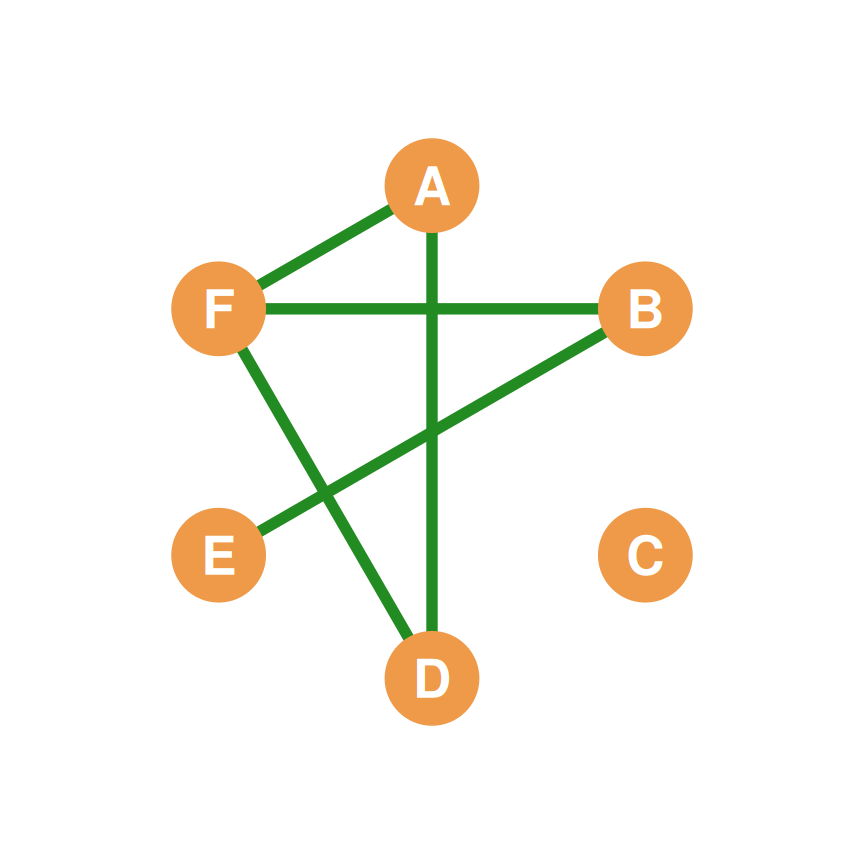
Visualizing the Hadamard Product (\(\mathbf{P} \circ \mathbf{G}\))

Parties and Plays Games With

A B C D E F
A -- 1 0 0 1 0
B 1 -- 1 0 0 0
C 0 1 -- 1 0 0
D 0 0 1 -- 1 0
E 1 0 0 1 -- 1
F 0 0 0 0 1 --
  • Retains only the shared ties.
  • All uniplex ties are erased, leaving a sparse overlap network.
Part 2: The Matrix Transpose & Directed Graphs

Row and Column Sums

The most basic operation on a matrix: add up its rows and columns.

Adjacency Matrix \(\mathbf{P}\)

A B C D E F
A -- 1 1 0 1 0
B 1 -- 1 1 0 0
C 1 1 -- 1 1 1
D 0 1 1 -- 1 0
E 1 0 1 1 -- 1
F 0 0 1 0 1 --
  • The diagonal is all \(0\)s (no self-ties).

Parties With (\(\mathbf{P}\))
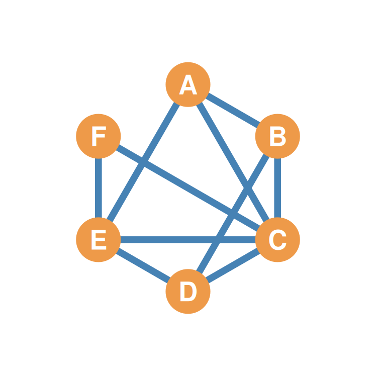
  • Row sum of node \(i\): \(\sum_j a_{ij}\) — pick a row, add across the columns.
  • Column sum of node \(j\): \(\sum_i a_{ij}\) — pick a column, add down the rows.
  • For a symmetric (undirected) adjacency matrix, the row and column sums are identical — they give each node’s degree (worked out on the next slide).
  • In directed graphs they differ — more on that in two slides.

Working the Example: The Undirected Case (\(\mathbf{P}\))

Adjacency Matrix \(\mathbf{P}\)

A B C D E F
A -- 1 1 0 1 0
B 1 -- 1 1 0 0
C 1 1 -- 1 1 1
D 0 1 1 -- 1 0
E 1 0 1 1 -- 1
F 0 0 1 0 1 --

Row sums for every node:

A B C D E F
3 3 5 3 4 2

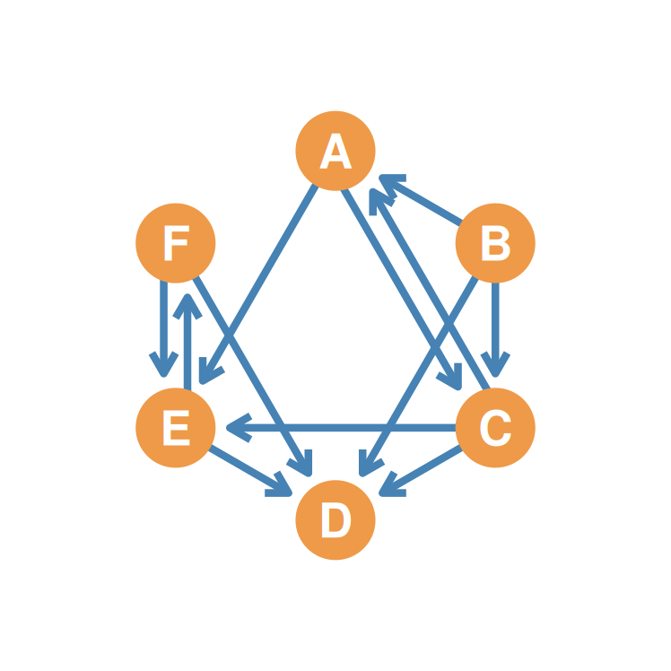
The Parties With Graph (\(\mathbf{P}\))
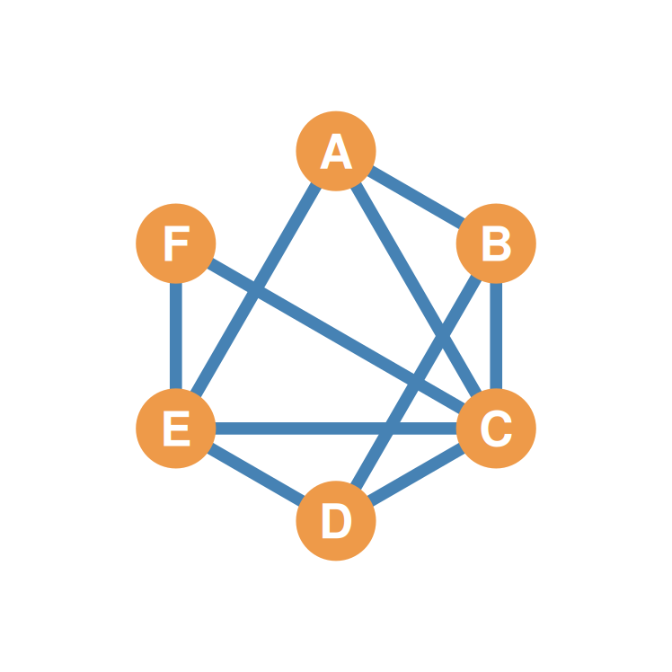
Row sum of node C — add across row C, cell by cell:

\[a_{CA} + a_{CB} + a_{CC} + a_{CD} + a_{CE} + a_{CF}\] \[= \color{red}{1} + \color{red}{1} + 0 + \color{red}{1} + \color{red}{1} + \color{red}{1} = \mathbf{5}\]

  • \(\mathbf{P}\) is symmetric (\(p_{ij} = p_{ji}\)): adding down column C reads the same numbers right back — the column sum is also \(\mathbf{5}\).
  • With undirected ties, every tie of C’s shows up once in C’s row and once in C’s column — so row sum = column sum, always.
  • That common sum is C’s degree (C parties with A, B, D, E, F). Doing it for every node (table at left) recovers all the degrees.

Working the Example: Row Sums (Directed)

Adjacency Matrix \(\mathbf{A}\)

A B C D E F
A -- 0 1 0 1 0
B 1 -- 1 1 0 0
C 1 0 -- 1 1 0
D 0 0 0 -- 0 0
E 0 0 0 1 -- 1
F 0 0 0 1 1 --

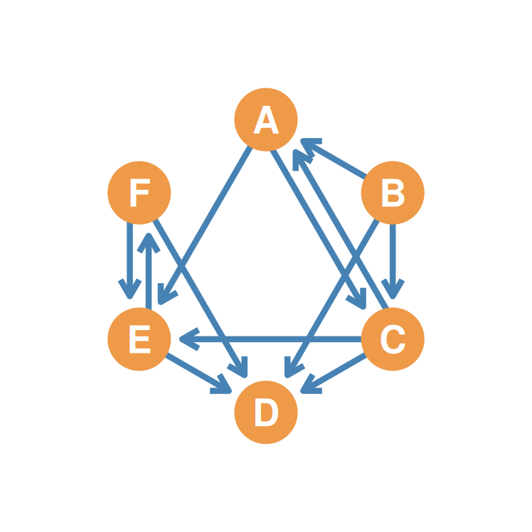
The Directed Graph (\(\mathbf{A}\))

Row sum of node B — add across row B, cell by cell:

\[a_{BA} + a_{BB} + a_{BC} + a_{BD} + a_{BE} + a_{BF}\] \[= \color{red}{1} + 0 + \color{red}{1} + \color{red}{1} + 0 + 0 = \mathbf{3}\]

  • Each cell \(a_{Bj}\) reads “B ties to \(j\)” — the first subscript is fixed at B, the second runs over every column.
  • The highlighted cells are exactly the ties B sends (its row): B is a pure sender.
  • Shorthand: \(\sum_j a_{Bj}\) — the summation sign does the “cell by cell” walking for us.

Working the Example: Column Sums (Directed)

Adjacency Matrix \(\mathbf{A}\)

A B C D E F
A -- 0 1 0 1 0
B 1 -- 1 1 0 0
C 1 0 -- 1 1 0
D 0 0 0 -- 0 0
E 0 0 0 1 -- 1
F 0 0 0 1 1 --

The Directed Graph (\(\mathbf{A}\))

Column sum of node D — add down column D, cell by cell:

\[a_{AD} + a_{BD} + a_{CD} + a_{DD} + a_{ED} + a_{FD}\] \[= 0 + \color{red}{1} + \color{red}{1} + 0 + \color{red}{1} + \color{red}{1} = \mathbf{4}\]

  • Each cell \(a_{iD}\) reads “\(i\) ties to D” — the second subscript is fixed at D, the first runs over every row.
  • The highlighted cells are exactly the ties D receives (its column): D is a pure receiver.
  • Shorthand: \(\sum_i a_{iD}\).

Row and Column Sums: Outdegrees and Indegrees

Row Sums = Outdegree

A B C D E F
2 3 3 0 2 2
  • Summing across a row counts the ties node \(i\) sends to others: \(i\)’s outdegree.

Column Sums = Indegree

A B C D E F
2 0 2 4 3 1
  • Summing down a column counts the ties node \(j\) receives from others: \(j\)’s indegree.

Directed Graph (\(\mathbf{A}\))
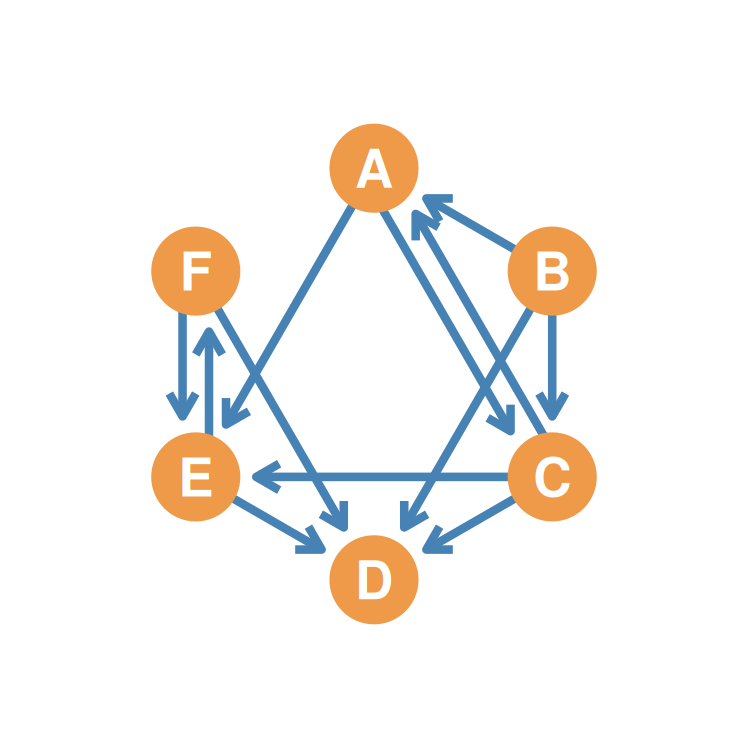
  • Node B: outdegree 3, indegree 0 — a pure sender (ties to A, C, D; nobody ties to B).
  • Node D: indegree 4, outdegree 0 — a pure receiver (B, C, E, F all tie to D; D ties to no one).

The Matrix Transpose (\(\mathbf{A}^T\))

  • The Transpose of a matrix \(\mathbf{A}\) is the same matrix with its rows and columns flipped:
    • Written as \(\mathbf{A}^T\) or \(\mathbf{A}'\).
    • The Rule: Row \(i\) of the original matrix becomes Column \(i\) of the transpose.
    • Formally: \(a^T_{ij} = a_{ji}\) for all cells.
  • Symmetric vs. Asymmetric Adjacency Matrices:
    • For undirected graphs, relationships are reciprocal by definition, so the matrix is symmetric (\(\mathbf{A}^T = \mathbf{A}\)).
    • For directed graphs (digraphs), ties can be one-way, resulting in an asymmetric matrix (\(\mathbf{A}^T \neq \mathbf{A}\)).

Clarification: Why Transpose Matters for Directed Networks

The transpose reverses the direction of every tie:

  • Original matrix \(\mathbf{A}\): If \(a_{ij} = 1\), person \(i\) sends a tie to person \(j\) (directional).
  • Transposed matrix \(\mathbf{A}^T\): If \(a^T_{ij} = a_{ji}\), we now read \(j\)’s tie to \(i\) at position \([i,j]\).

Example: - In \(\mathbf{A}\): A → B (row 1, col 2) = 1 - In \(\mathbf{A}^T\): B → A (row 2, col 1) becomes row 1, col 2 = 1 - The direction is reversed.

This is essential for finding mutual ties (cells where both \(a_{ij} = 1\) AND \(a_{ji} = 1\), which we can identify by comparing \(\mathbf{A}\) and \(\mathbf{A}^T\)).

Visualizing the Matrix Transpose

Matrix \(\mathbf{A}\)

A B C D E F
A -- 0 1 0 1 0
B 1 -- 1 1 0 0
C 1 0 -- 1 1 0
D 0 0 0 -- 0 0
E 0 0 0 1 -- 1
F 0 0 0 1 1 --
  • Row 1 of \(\mathbf{A}\) (0, 0, 1, 0, 1, 0) is Column 1 of \(\mathbf{A}^T\).
  • Rule: Row \(i\) of \(\mathbf{A}\) becomes Column \(i\) of \(\mathbf{A}^T\).

Transpose \(\mathbf{A}^T\)

A B C D E F
A -- 1 1 0 0 0
B 0 -- 0 0 0 0
C 1 1 -- 0 0 0
D 0 1 1 -- 1 1
E 1 0 1 0 -- 1
F 0 0 0 0 1 --
  • Flipped horizontally: rows become columns.
  • Reverses the direction of every single arrow in the network.

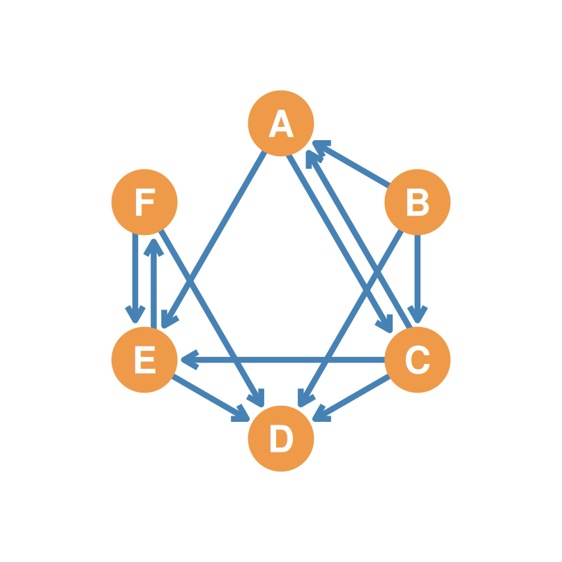
Directed Graph (\(\mathbf{A}\))
The Transpose as a Reversed Graph

  • \(\mathbf{A}^T\) is not just a table trick — it’s a different network: the same six people, with every arrow reversed.
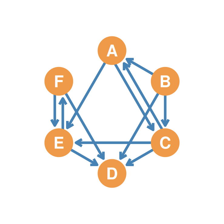
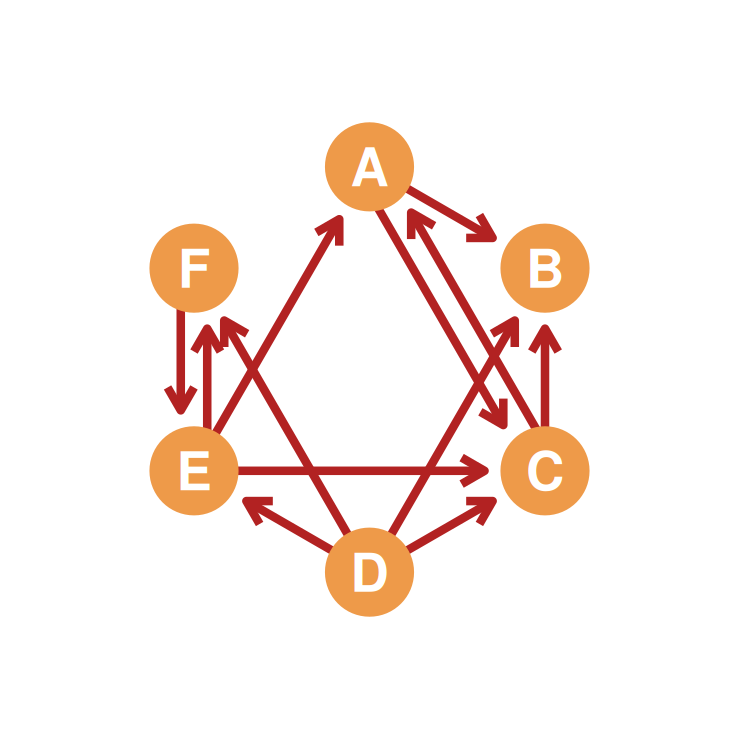
  • Check a pair: in \(\mathbf{A}\) (left), B sends to A; in \(\mathbf{A}^T\) (right), A sends to B.
  • Sender and receiver swap roles: outdegrees of \(\mathbf{A}\) become the indegrees of \(\mathbf{A}^T\), and vice versa.

Part 3: Directed Dyads & The Dyad Census

Dyads in Directed Graphs

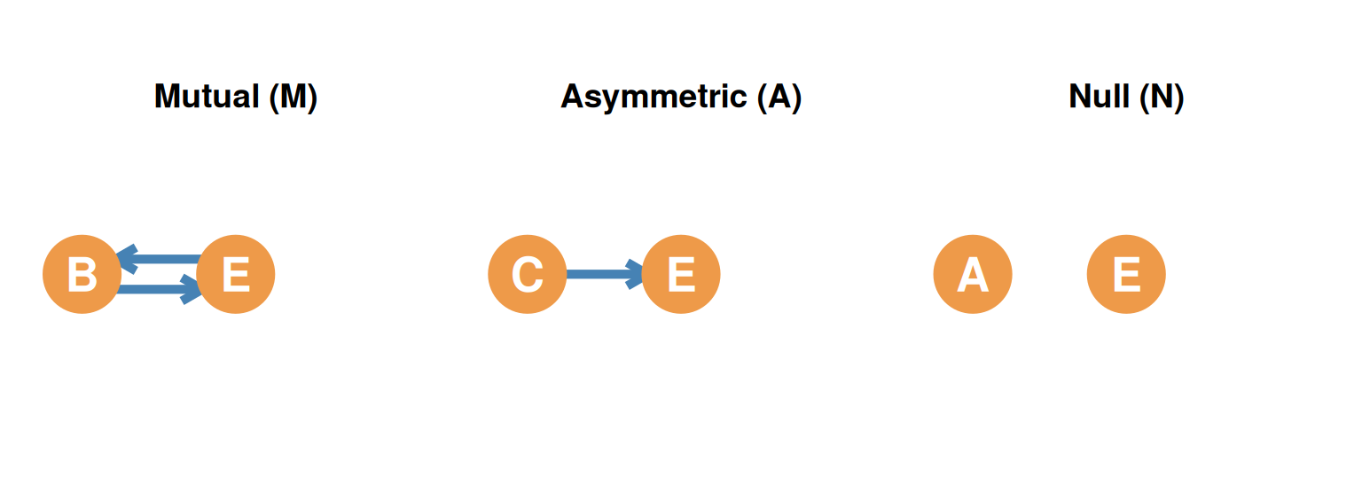
  • In a directed graph, any pair of nodes (a dyad) can have one of three configurations:
    1. Mutual (M): Both directed edges are present (\(i \leftrightarrow j\)).
    2. Asymmetric (A): Only one directed edge is present (\(i \rightarrow j\) or \(j \rightarrow i\)).
    3. Null (N): Neither directed edge is present (disconnected).
  • An easy way to remember these three types of dyads is the mnemonic MAN (Mutual, Asymmetric, Null).
The Dyad Census

Adjacency Matrix \(\mathbf{A}\)

A B C D E F
A -- 0 1 0 1 0
B 1 -- 1 1 0 0
C 1 0 -- 1 1 0
D 0 0 0 -- 0 0
E 0 0 0 1 -- 1
F 0 0 0 1 1 --
  • The diagonal is all \(0\)s (no self-ties).

The Directed Graph (\(\mathbf{A}\))
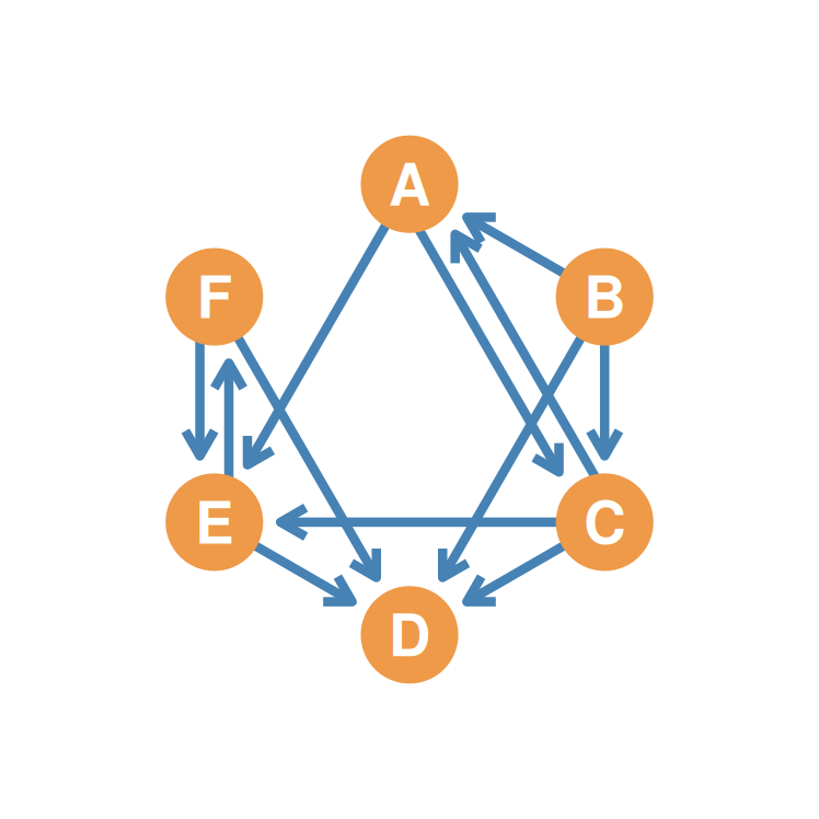
  • The Dyad Census is a count of the total number of Mutuals (\(N_M\)), Asymmetrics (\(N_A\)), and Nulls (\(N_N\)) in a directed graph.
  • We compute these counts with cell-by-cell matrix operations (Hadamard product and subtraction) on \(\mathbf{A}\) (left) and \(\mathbf{A}^T\).
  • We will perform these calculations on our 6-node directed reference graph (middle):
    • \(N_M\) = number of mutual dyads
    • \(N_A\) = number of asymmetric dyads
    • \(N_N\) = number of null dyads

1. Mutual Dyads Matrix (\(\mathbf{M} = \mathbf{A} \circ \mathbf{A}^T\)): Setup

  • Multiplying \(\mathbf{A}\) by its transpose \(\mathbf{A}^T\) element-wise extracts only mutual dyads where \(a_{ij}=1\) and \(a_{ji}=1\):

\[\mathbf{M} = \mathbf{A} \circ \mathbf{A}^T = \begin{pmatrix} 0 & 0 & 1 & 0 & 1 & 0 \\ 1 & 0 & 1 & 1 & 0 & 0 \\ 1 & 0 & 0 & 1 & 1 & 0 \\ 0 & 0 & 0 & 0 & 0 & 0 \\ 0 & 0 & 0 & 1 & 0 & 1 \\ 0 & 0 & 0 & 1 & 1 & 0 \end{pmatrix} \circ \begin{pmatrix} 0 & 1 & 1 & 0 & 0 & 0 \\ 0 & 0 & 0 & 0 & 0 & 0 \\ 1 & 1 & 0 & 0 & 0 & 0 \\ 0 & 1 & 1 & 0 & 1 & 1 \\ 1 & 0 & 1 & 0 & 0 & 1 \\ 0 & 0 & 0 & 0 & 1 & 0 \end{pmatrix}\]

1. Mutual Dyads Matrix (\(\mathbf{M} = \mathbf{A} \circ \mathbf{A}^T\)): Calculation

  • We multiply the corresponding cells of \(\mathbf{A}\) and \(\mathbf{A}^T\) element-wise:

\[\mathbf{M} = \begin{pmatrix} 0\times0 & 0\times1 & 1\times1 & 0\times0 & 1\times0 & 0\times0 \\ 1\times0 & 0\times0 & 1\times0 & 1\times0 & 0\times0 & 0\times0 \\ 1\times1 & 0\times1 & 0\times0 & 1\times0 & 1\times0 & 0\times0 \\ 0\times0 & 0\times1 & 0\times1 & 0\times0 & 0\times1 & 0\times1 \\ 0\times1 & 0\times0 & 0\times1 & 1\times0 & 0\times0 & 1\times1 \\ 0\times0 & 0\times0 & 0\times0 & 1\times0 & 1\times1 & 0\times0 \end{pmatrix} = \begin{pmatrix} - & 0 & \mathbf{1} & 0 & 0 & 0 \\ 0 & - & 0 & 0 & 0 & 0 \\ \mathbf{1} & 0 & - & 0 & 0 & 0 \\ 0 & 0 & 0 & - & 0 & 0 \\ 0 & 0 & 0 & 0 & - & \mathbf{1} \\ 0 & 0 & 0 & 0 & \mathbf{1} & - \end{pmatrix}\]

1. Mutual Dyads Matrix (\(\mathbf{M} = \mathbf{A} \circ \mathbf{A}^T\)): Result

Census Count (\(N_M\))

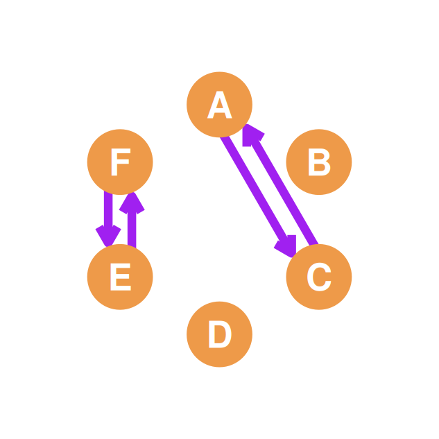
  • Only reciprocal ties are kept (A-C and E-F).
  • Sum of cells in \(\mathbf{M}\) is 4.
  • \[N_M = \frac{\sum M_{ij}}{2} = \frac{4}{2} = \mathbf{2} \text{ mutual dyads}\]

Matrix Result (\(\mathbf{M}\))

A B C D E F
A -- 0 1 0 0 0
B 0 -- 0 0 0 0
C 1 0 -- 0 0 0
D 0 0 0 -- 0 0
E 0 0 0 0 -- 1
F 0 0 0 0 1 --

Mutual ties graph

2. Asymmetric Dyads Matrix (\(\mathbf{S} = \mathbf{A} \circ (\mathbf{1} - \mathbf{A}^T)\)): Setup

  • Multiplying \(\mathbf{A}\) by the complement of transpose (\(\mathbf{1} - \mathbf{A}^T\)) extracts unreciprocated ties:

\[\mathbf{S} = \mathbf{A} \circ (\mathbf{1} - \mathbf{A}^T) = \begin{pmatrix} 0 & 0 & 1 & 0 & 1 & 0 \\ 1 & 0 & 1 & 1 & 0 & 0 \\ 1 & 0 & 0 & 1 & 1 & 0 \\ 0 & 0 & 0 & 0 & 0 & 0 \\ 0 & 0 & 0 & 1 & 0 & 1 \\ 0 & 0 & 0 & 1 & 1 & 0 \end{pmatrix} \circ \begin{pmatrix} - & 0 & 0 & 1 & 1 & 1 \\ 1 & - & 1 & 1 & 1 & 1 \\ 0 & 0 & - & 1 & 1 & 1 \\ 1 & 0 & 0 & - & 0 & 0 \\ 0 & 1 & 0 & 1 & - & 0 \\ 1 & 1 & 1 & 1 & 0 & - \end{pmatrix}\]

2. Asymmetric Dyads Matrix (\(\mathbf{S} = \mathbf{A} \circ (\mathbf{1} - \mathbf{A}^T)\)): Calculation

  • We multiply the corresponding cells of \(\mathbf{A}\) and \((\mathbf{1} - \mathbf{A}^T)\) element-wise:
\[\mathbf{S} = \begin{pmatrix} 0\times- & 0\times0 & 1\times0 & 0\times1 & 1\times1 & 0\times1 \\ 1\times1 & 0\times- & 1\times1 & 1\times1 & 0\times1 & 0\times1 \\ 1\times0 & 0\times0 & 0\times- & 1\times1 & 1\times1 & 0\times1 \\ 0\times1 & 0\times0 & 0\times0 & 0\times- & 0\times0 & 0\times0 \\ 0\times0 & 0\times1 & 0\times0 & 1\times1 & 0\times- & 1\times0 \\ 0\times1 & 0\times1 & 0\times1 & 1\times1 & 1\times0 & 0\times- \end{pmatrix} = \begin{pmatrix} - & 0 & 0 & 0 & \mathbf{1} & 0 \\ \mathbf{1} & - & \mathbf{1} & \mathbf{1} & 0 & 0 \\ 0 & 0 & - & \mathbf{1} & \mathbf{1} & 0 \\ 0 & 0 & 0 & - & 0 & 0 \\ 0 & 0 & 0 & \mathbf{1} & - & 0 \\ 0 & 0 & 0 & \mathbf{1} & 0 & - \end{pmatrix}\]

2. Asymmetric Dyads Matrix (\(\mathbf{S} = \mathbf{A} \circ (\mathbf{1} - \mathbf{A}^T)\)): Result

Census Count (\(N_A\))

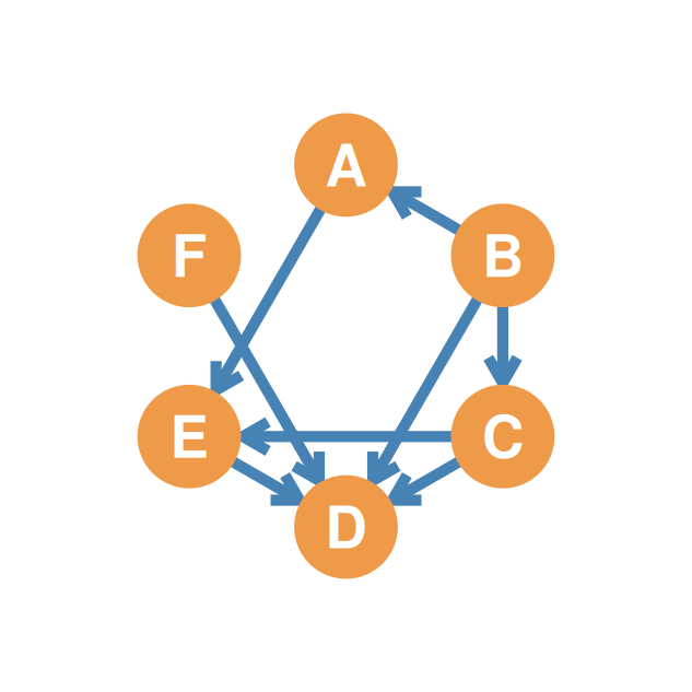
  • Retains only unreciprocated outgoing ties.
  • Sum of cells in \(\mathbf{S}\) is 8.
  • \[N_A = \sum S_{ij} = \mathbf{8} \text{ asymmetric dyads}\]

Matrix Result (\(\mathbf{S}\))

A B C D E F
A -- 0 0 0 1 0
B 1 -- 1 1 0 0
C 0 0 -- 1 1 0
D 0 0 0 -- 0 0
E 0 0 0 1 -- 0
F 0 0 0 1 0 --

Asymmetric ties graph

3. Null Dyads Matrix (\(\mathbf{N} = (\mathbf{1} - \mathbf{A}) \circ (\mathbf{1} - \mathbf{A}^T)\)): Setup

  • Multiplying the complement of \(\mathbf{A}\) by the complement of transpose (\(\mathbf{1} - \mathbf{A}^T\)) extracts completely disconnected dyads:

\[\mathbf{N} = (\mathbf{1} - \mathbf{A}) \circ (\mathbf{1} - \mathbf{A}^T) = \begin{pmatrix} - & 1 & 0 & 1 & 0 & 1 \\ 0 & - & 0 & 0 & 1 & 1 \\ 0 & 1 & - & 0 & 0 & 1 \\ 1 & 1 & 1 & - & 1 & 1 \\ 1 & 1 & 1 & 0 & - & 0 \\ 1 & 1 & 1 & 0 & 0 & - \end{pmatrix} \circ \begin{pmatrix} - & 0 & 0 & 1 & 1 & 1 \\ 1 & - & 1 & 1 & 1 & 1 \\ 0 & 0 & - & 1 & 1 & 1 \\ 1 & 0 & 0 & - & 0 & 0 \\ 0 & 1 & 0 & 1 & - & 0 \\ 1 & 1 & 1 & 1 & 0 & - \end{pmatrix}\]

3. Null Dyads Matrix (\(\mathbf{N} = (\mathbf{1} - \mathbf{A}) \circ (\mathbf{1} - \mathbf{A}^T)\)): Calculation

  • We multiply the corresponding cells of \((\mathbf{1} - \mathbf{A})\) and \((\mathbf{1} - \mathbf{A}^T)\) element-wise:
\[\mathbf{N} = \begin{pmatrix} -\times- & 1\times0 & 0\times0 & 1\times1 & 0\times1 & 1\times1 \\ 0\times1 & -\times- & 0\times1 & 0\times1 & 1\times1 & 1\times1 \\ 0\times0 & 1\times0 & -\times- & 0\times1 & 0\times1 & 1\times1 \\ 1\times1 & 1\times0 & 1\times0 & -\times- & 1\times0 & 1\times0 \\ 1\times0 & 1\times1 & 1\times0 & 0\times1 & -\times- & 0\times0 \\ 1\times1 & 1\times1 & 1\times1 & 0\times1 & 0\times0 & -\times- \end{pmatrix}\] \[= \begin{pmatrix} - & 0 & 0 & \mathbf{1} & 0 & \mathbf{1} \\ 0 & - & 0 & 0 & \mathbf{1} & \mathbf{1} \\ 0 & 0 & - & 0 & 0 & \mathbf{1} \\ \mathbf{1} & 0 & 0 & - & 0 & 0 \\ 0 & \mathbf{1} & 0 & 0 & - & 0 \\ \mathbf{1} & \mathbf{1} & \mathbf{1} & 0 & 0 & - \end{pmatrix}\]

3. Null Dyads Matrix (\(\mathbf{N} = (\mathbf{1} - \mathbf{A}) \circ (\mathbf{1} - \mathbf{A}^T)\)): Result

Census Count (\(N_N\))

  • Retains completely disconnected dyads.
  • Sum of cells in \(\mathbf{N}\) is 10.
  • \[N_N = \frac{\sum N_{ij}}{2} = \frac{10}{2} = \mathbf{5} \text{ null dyads}\]

Matrix Result (\(\mathbf{N}\))

A B C D E F
A -- 0 0 1 0 1
B 0 -- 0 0 1 1
C 0 0 -- 0 0 1
D 1 0 0 -- 0 0
E 0 1 0 0 -- 0
F 1 1 1 0 0 --

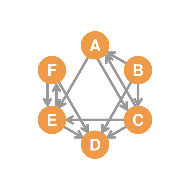
Reference Graph (A)

The Dyad Census Identity Check

  • In any directed graph of size \(n\), the total number of dyads (pairs) is \(\frac{n(n-1)}{2}\).
  • For our \(n=6\) graph, we must have exactly \(\frac{6 \times 5}{2} = 15\) dyads.
  • Check:
    • \(N_M + N_A + N_N = 2 + 8 + 5 = \mathbf{15}\)
    • The mathematics accounts for every single pair in the network perfectly!
  • The Matrix Identity:
    • The cell-wise sum of our three matrices always equals the complete graph minus the diagonal (\(\mathbf{J} - \mathbf{I}\)):
    • \(\mathbf{M} + \mathbf{S} + \mathbf{N} = \mathbf{J} - \mathbf{I}\)

Graph Reciprocity (\(R\))

  • Graph Reciprocity (\(R\)) measures the extent to which a directed graph approximates the ideal of complete reciprocity.
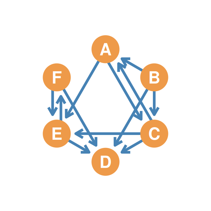
  • It is defined as the proportion of connected dyads that are mutual: \[R = \frac{N_M}{N_M + N_A}\]
  • Calculation:
    • We know \(N_M = 2\) and \(N_A = 8\).
    • \(R = \frac{2}{2 + 8} = \frac{2}{10} = \mathbf{0.20}\)

The Directed Graph (\(\mathbf{A}\))
Clarification: Interpreting Graph Reciprocity

  • Range: \(R\) always falls between 0 and 1.
    • \(R = 1\): Perfect reciprocity — all connected dyads are mutual (trust, equality).
    • \(R = 0\): Complete asymmetry — all connections are one-way (hierarchy, dominance).
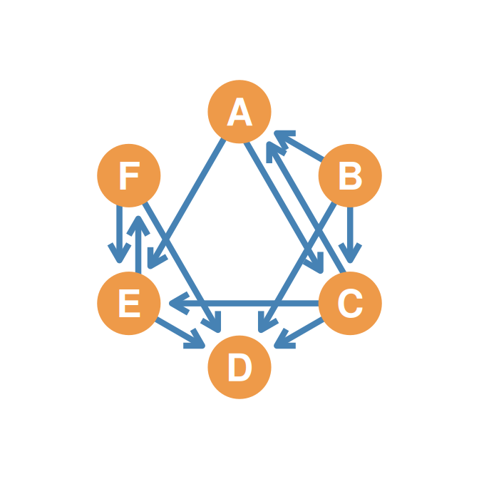
    • \(R = 0.20\): This network (right) has low reciprocity — only 20% of connected pairs reciprocate ties.

Sociological Meaning: - High \(R\) suggests trust-based, egalitarian social structures (friendships, partnerships). - Low \(R\) suggests hierarchical or competitive structures (respect, followers, citations).

The Directed Graph (\(\mathbf{A}\))
Summary: Part I

You now understand: - Basic operations (Addition, Complement, Hadamard) combine or filter relationship types. - The Transpose flips directions; essential for directed networks. - The Dyad Census classifies all pairs into Mutual, Asymmetric, or Null categories using matrix operations. - Graph Reciprocity summarizes the balance between mutual and one-way ties.

Next session: Standard matrix multiplication, conformability, and dynamic applications (paths, walks, clustering).