Graph Theory: Equivalence & Similarity

The Positional Structure of Social Networks

Part 1: The Positional Approach & Structural Equivalence

The Position Approach

  • In social network analysis, we can partition nodes using two different philosophies:
    1. The Group Approach: Nodes are divided into subsets that are tightly interconnected with one another.
    2. The Positional Approach: Nodes are divided into subsets based on how similar they are in their patterns of connectivity with others.
  • Nodes in the same positional class are said to occupy the same position or role in the social structure.
  • We distinguish between:
    • Structural Equivalence: Nodes are connected to the exact same other nodes.
    • Regular Equivalence: Nodes are connected to equivalent others (e.g., all teachers are connected to students, even if they are different students).

Defining Structural Equivalence

  • Structural Equivalence (Lorrain & White, 1971):
    • Two nodes are structurally equivalent if they are connected to the same other nodes.
    • Their patterns of connectivity are mathematically identical.
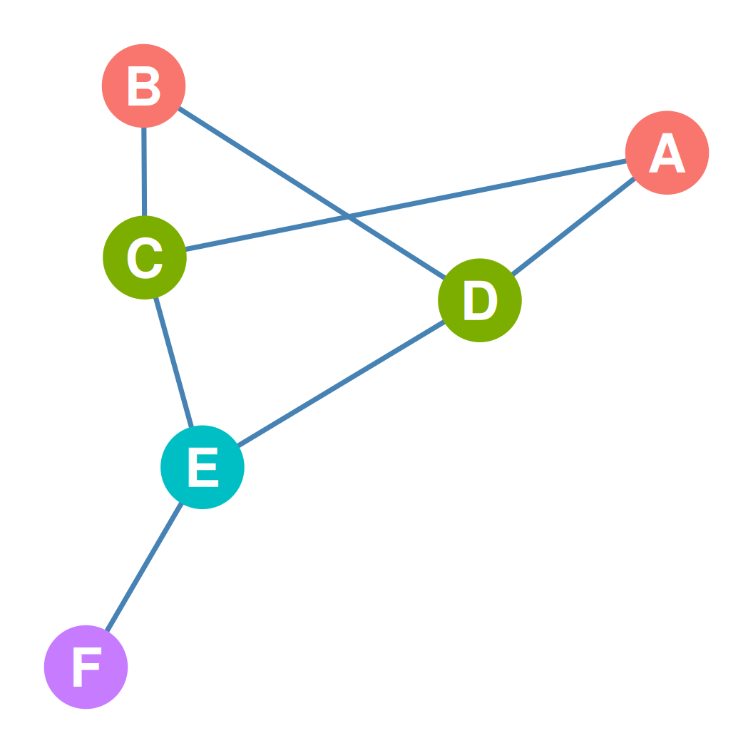
    • In the graph on the right:
      • \(\{C, D\}\) are structurally equivalent because both are connected to \(\{A, B, E\}\).
      • \(\{A, B\}\) are structurally equivalent because both are connected to \(\{C, D\}\).
      • \(\{E\}\) and \(\{F\}\) occupy unique positions (neighborhoods are not shared).

Adjacency Matrix of Equivalent Positions

A B C D E F
A 0 0 1 1 0 0
B 0 0 1 1 0 0
C 1 1 0 0 1 0
D 1 1 0 0 1 0
E 0 0 1 1 0 1
F 0 0 0 0 1 0
  • Structurally equivalent nodes have identical rows (and columns) in the adjacency matrix.
  • Rows A and B are identical (\(0, 0, 1, 1, 0, 0\)), as are Rows C and D (\(1, 1, 0, 0, 1, 0\)).
  • Nodes in unique positions (like \(E\) and \(F\)) have completely unique row patterns.

Structural Similarity: A Necessary Relaxation

  • In real-world social networks, strict structural equivalence is extremely rare.
    • It only allows a binary “yes” or “no” answer: either nodes connect to the exact same neighbors, or they do not.
    • If node \(A\) and node \(B\) share 99 out of 100 neighbors, they are technically not structurally equivalent!
  • Structural Similarity:
    • Allows for a “more or less” gradient rather than binary classification.
    • Measures the extent to which two nodes have highly overlapping patterns of connectivity.
    • Let’s look at how we measure this.

Part 2: Measuring Structural Similarity

Euclidean Distance (\(d^{Euclid}_{k,l}\))

  • Ronald Burt (1976) proposed measuring structural similarity by calculating the Euclidean Distance between the row vectors of nodes in the adjacency matrix.
  • For nodes \(k\) and \(l\), the distance is:
    • \[d^{Euclid}_{k,l} = \sqrt{\sum_j (a_{(k)j} - a_{(l)j})^2}\]
  • Key Properties:
    • If nodes are structurally equivalent, their Euclidean distance is exactly zero.
    • The larger the distance, the less structurally similar the two nodes are.

Euclidean Distance Calculation: \(A\) vs. \(C\)

  • Let’s calculate the Euclidean distance between \(A\) (\(0, 0, 1, 1, 0, 0\)) and \(C\) (\(1, 1, 0, 0, 1, 0\)):
Vector A 0 0 1 1 0 0
Vector C 1 1 0 0 1 0
A - C (0 - 1) (0 - 1) (1 - 0) (1 - 0) (0 - 1) (0 - 0)
Difference -1 -1 1 1 -1 0
Squared Diff 1 1 1 1 1 0
  • Sum of squared differences: \(\sum_j (a_{(A)j} - a_{(C)j})^2 = 1 + 1 + 1 + 1 + 1 + 0 = 5\)
  • Euclidean Distance: \(d^{Euclid}_{A, C} = \sqrt{5} \approx 2.24\)

The Structural Similarity Matrix (\(S\))

A B C D E F
A -- 0 2.24 2.24 1 1.73
B 0 -- 2.24 2.24 1 1.73
C 2.24 2.24 -- 0 2.45 1.41
D 2.24 2.24 0 -- 2.45 1.41
E 1 1 2.45 2.45 -- 2
F 1.73 1.73 1.41 1.41 2 --
  • Pairs of structurally equivalent nodes (\(\{A, B\}\) and \(\{C, D\}\)) have a distance of 0.00.
  • Unique positions like \(F\) have high distances to almost everyone else (e.g., \(d_{A, F} = 2.45\)).

Euclidean Distance in Directed Graphs

  • When networks contain asymmetric (directed) ties, we must distinguish between two behaviors:
    1. Sending Ties: Do nodes \(u\) and \(v\) point to the same out-neighbors? (Row similarity)
    2. Receiving Ties: Do nodes \(u\) and \(v\) receive ties from the same in-neighbors? (Column similarity)
  • Two directed nodes are structurally equivalent if and only if they send ties to the same others and receive ties from the same others.
  • The Euclidean distance formula expands to sum both row and column differences:
    • \[d^{Euclidean}_{k,l} = \sqrt{\sum_j (a_{(k)j}-a_{(l)j})^2 + \sum_i (a_{(k)i}-a_{(l)i})^2}\]

Directed Similarity Example

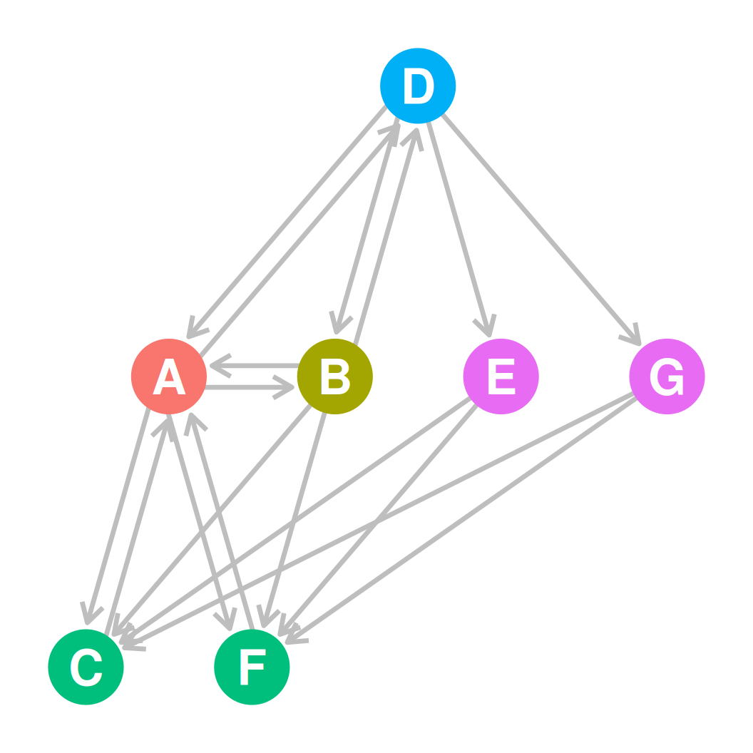
  • Consider the directed graph on the right.
  • Nodes with the same color are structurally equivalent under directed Euclidean distance:
    • \(\{E, G\}\) are structurally equivalent (\(d_{E, G} = 0\)). They send ties to \(\{C, F\}\) and receive ties from \(\{D\}\).
    • \(\{C, F\}\) are structurally equivalent (\(d_{C, F} = 0\)). They send ties to \(\{A\}\) and receive ties from \(\{A, B, E, G\}\).
    • Structural equivalence in directed networks elegantly maps actors into identical social roles.
Part 3: Measuring Similarity via Neighborhood Overlap

The Intuition of Neighborhood Overlap

  • Recall that the neighborhood of a node is the set of all other nodes adjacent to it.
  • Neighborhood Overlap:
    • The more neighbors two nodes have in common, the more structurally similar they are.
    • If you and your colleague share 100% of your friends, you are structurally equivalent.
    • If you share none of your friends, you occupy completely different social worlds.
  • We can formalize this overlap using three classical set-theoretic coefficients.

Three Classical Coefficients

  • Let \(n_{ij}\) be the number of common neighbors of nodes \(i\) and \(j\); let \(k_i\) and \(k_j\) be their degrees.

1. Jaccard Similarity

\[J_{ij} = \frac{n_{ij}}{k_i + k_j - n_{ij}}\]

2. Dice Similarity

\[D_{ij} = \frac{2n_{ij}}{k_i + k_j}\]

3. Cosine Similarity

\[C_{ij} = \frac{n_{ij}}{\sqrt{k_i k_j}}\]

  • All three metrics range from 0.0 (no overlap) to 1.0 (structural equivalence).

Comparing Overlap Matrices

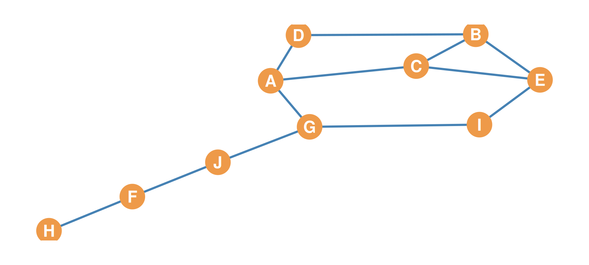
Cosine Similarity Matrix Example

A B C D E F G H I J
A -- 0.67 0 0 0.33 0 0 0 0.41 0.41
B -- -- 0.33 0 0.33 0 0 0 0.41 0
C -- -- -- 0.82 0.33 0 0.33 0 0.41 0
D -- -- -- -- 0.41 0 0.41 0 0 0
E -- -- -- -- -- 0 0.33 0 0 0
F -- -- -- -- -- -- 0.41 0 0 0
G -- -- -- -- -- -- -- 0 0 0
H -- -- -- -- -- -- -- -- 0 0.71
I -- -- -- -- -- -- -- -- -- 0.5
J -- -- -- -- -- -- -- -- -- --
  • Cells record Cosine Similarity between node neighborhoods.
  • If \(C_{ij} = 0.00\), \(i\) and \(j\) share absolutely zero friends.
  • If \(C_{ij} = 1.00\), \(i\) and \(j\) are structurally equivalent.

Neighborhood Overlap in Directed Graphs

  • In directed networks, neighborhood overlap splits into:
    • Out-Similarity: Overlap in outgoing ties (pointing to the same others).
    • In-Similarity: Overlap in incoming ties (receiving nominations from the same others).
  • In Citation Networks (where paper \(A \rightarrow B\) means \(A\) cites \(B\)):
    • Bibliographic Coupling (Out-Similarity):
      • The number of references two papers have in common.
      • Measures similarity in theoretical foundations or sources.
    • Co-Citation (In-Similarity):
      • The frequency with which two papers are cited together by subsequent papers.
      • Measures how much the scientific community associates their ideas.

Directed Cosine Equations

  • Let \(n_{ij}^{out}\) / \(n_{ij}^{in}\) be the shared out-/in-neighbors, and \(k_i^{out}\) / \(k_i^{in}\) the out-/in-degrees.
  • Cosine Out-Similarity:
    • \[C_{ij}^{out} = \frac{n_{ij}^{out}}{\sqrt{k_i^{out} k_j^{out}}}\]
  • Cosine In-Similarity:
    • \[C_{ij}^{in} = \frac{n_{ij}^{in}}{\sqrt{k_i^{in} k_j^{in}}}\]
  • These formulas partition networks by highly specific sender and receiver roles.

Part 4: Structural, Automorphic, and Regular Equivalence

Three Concepts of Equivalence

  • Beyond structural equivalence (sharing the exact same neighbors), there are three nested notions of relational position:
    1. Structural Equivalence: Identical neighborhoods (\(N(u) = N(v)\)). Highly strict, same-neighbor rule.
    2. Automorphic Equivalence: Globally symmetrical/interchangeable nodes. Nodes can be swapped without changing the graph structure.
    3. Regular Equivalence: Connection to equivalent others. Focuses on general roles (e.g., all doctors connect to patients).
  • The Nested Hierarchy:
    • \(\text{Structural} \subseteq \text{Automorphic} \subseteq \text{Regular}\)
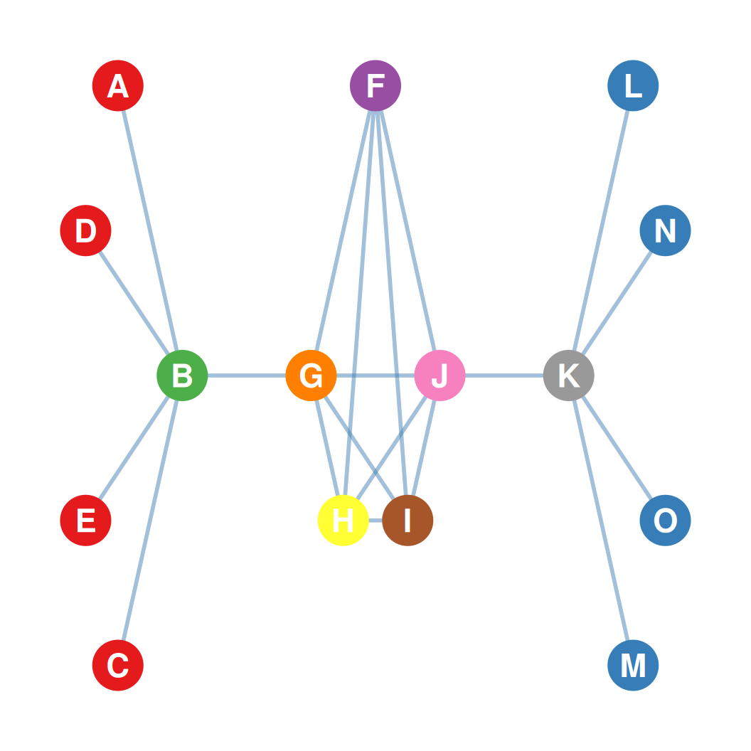
  • Let’s explore these definitions using a symmetrical 15-node network.

Symmetrical 15-Node Network

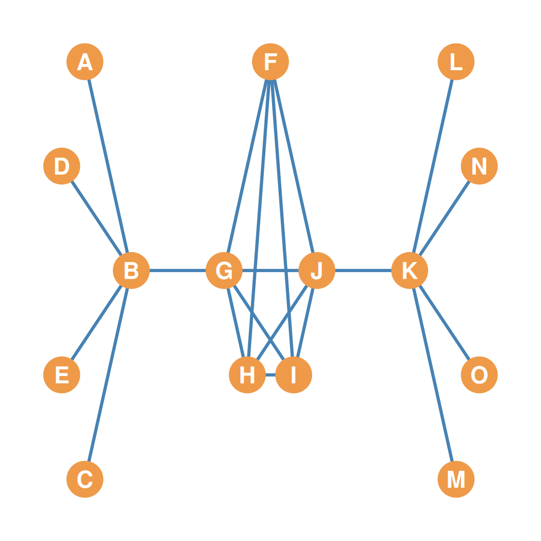
  • This 15-node network has:
    • Two star-like components centered at hubs \(B\) and \(K\).
    • Symmetrical leaf sets \(\{A,C,D,E\}\) and \(\{L,M,N,O\}\).
    • A tightly integrated central core \(\{F,G,H,I,J\}\).
    • \(G\) connects the core to hub \(B\); \(J\) connects the core to hub \(K\).
    • Let’s look at how we partition this network using the three equivalence criteria.
1. Structural Equivalence

  • Structural Equivalence Partition:
    • Requires connection to the exact same neighbors.
    • Groups:
      • Class 1: Leaf set \(\{A,C,D,E\}\) (connected only to \(B\)).
      • Class 2: Leaf set \(\{L,M,N,O\}\) (connected only to \(K\)).
      • All other nodes (colored separately) are in unique single-node classes.
    • Note: Symmetrical hubs \(B\) and \(K\) connect to different leaves, so they are not structurally equivalent!
2. Automorphic Equivalence

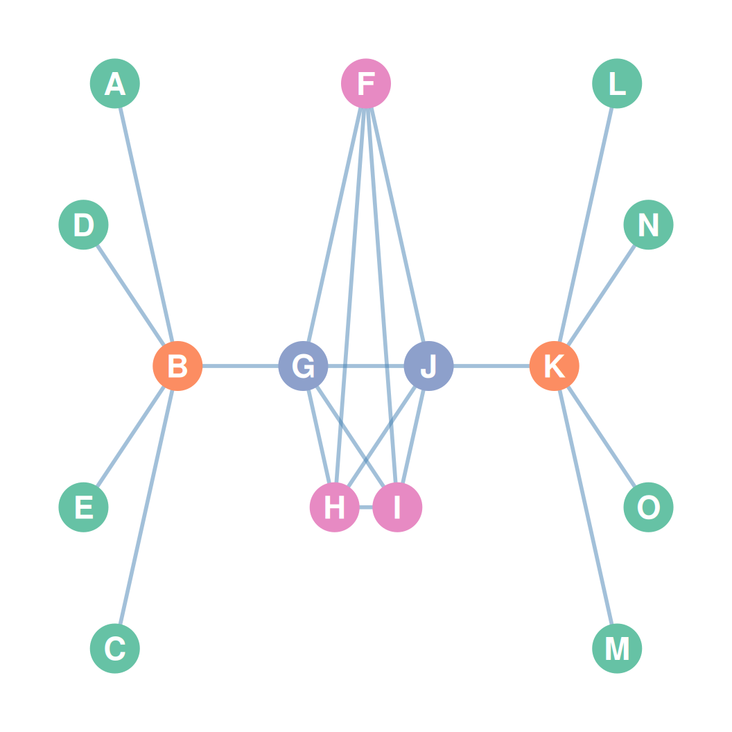
  • Automorphic Equivalence Partition:
    • Nodes that are globally interchangeable (symmetric swap).
    • groups nodes into four classes:
      • Leaves: \(\{A,C,D,E, L,M,N,O\}\)
      • Hubs: \(\{B,K\}\) (symmetric counterparts)
      • Core Bridges: \(\{G,J\}\) (gates to hubs)
      • Core Nodes: \(\{F,H,I\}\) (internally symmetric, no outside ties)
    • Successfully captures the structural similarity between hubs \(B\) and \(K\).
3. Regular Equivalence

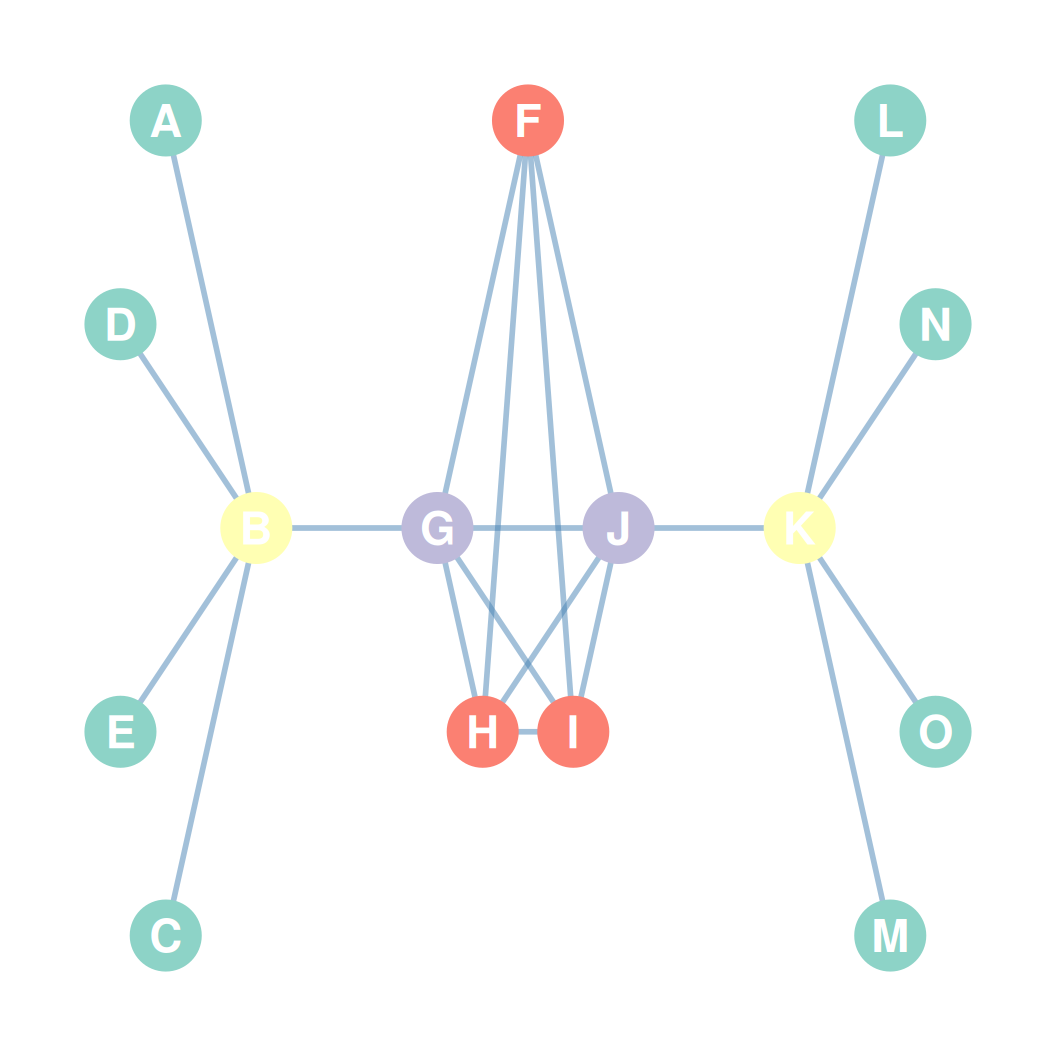
  • Regular Equivalence Partition:
    • Connects to equivalent others (general roles).
    • Groups the 15 nodes into four roles:
      • Class 1 (Leaves): \(\{A,C,D,E, L,M,N,O\}\) (connect only to Hubs)
      • Class 2 (Hubs): \(\{B,K\}\) (connect to Leaves and Core Bridges)
      • Class 3 (Core Bridges): \(\{G,J\}\) (connect to Hubs and Core nodes)
      • Class 4 (Core Nodes): \(\{F,H,I\}\) (connect to Core Bridges and Core nodes)
    • Elegant and highly flexible role-mapping.
Summary of Positional Concepts

  • Positions represent roles:
    • Unlike cohesive subgroups, actors do not need to connect to each other to be in the same position; they just need to connect to others similarly.
  • Structural Equivalence is the ideal limit:
    • Perfect row/column matching is highly elegant but rare in real social networks.
  • Structural Similarity relaxes the limit:
    • Distance metrics (Euclidean) and Overlap coefficients (Jaccard, Dice, Cosine) allow us to measure degrees of positional equivalence.
  • Directionality adds analytical depth:
    • Directed similarity splits into In-Similarity (Co-citation) and Out-Similarity (Bibliographic coupling), providing robust tools for citation and communication analysis.