Graph Theory: Sub-Groups & Cliques

The Cohesive Structures of Social Networks

Part 1: Subgroups

The Group Approach

  • The group level in networks sits in between:
    • the micro: dyads and triads
    • the macro: the “whole network”
  • Why groups?
    • Important functional units in organizations: workplaces, creative industries, science

The Group Approach

  • Why groups? Groups are the main units of solidarity and interaction in social systems:
    • Primary groups (family, support cliques)
    • Secondary groups (friends, workplaces, schools)
The Group Approach

  • Why groups? Groups are important sources of:
    • Ideational homogeneity
    • Conformity
    • Influence
    • Information transmission

The Group Approach

  • Questions:
    • How can we translate the concept of a group into network terms?
    • What are the most important group properties from a network perspective?
    • Cohesion, polarization, fragmentation

What are “groups”?

  • “Group” is a fuzzy social science concept, with many overlapping but sometimes contradictory verbal definitions.
  • As always, graph theory to the rescue!
  • The graph theoretic concept of a group is:
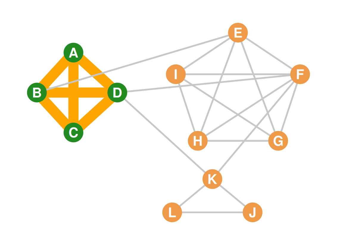
    • A relatively dense subgraph featuring more links among the subset of vertices that belong to the subgraph than links to vertices in the rest of the graph.
Graphs and subgraphs

  • A subgraph \(G' = (V', E')\) of a graph \(G = (V, E)\) exists when:
    • \(V'\) is a subset of \(V\) and \(E'\) is a subset of \(E\)
  • Many network methods are designed to split a graph into subgraphs
  • Subgraphs can be used to represent the social network concept of subgroup
Graphs and subgraphs

  • This is a subgraph!

Graphs and subgraphs

  • This is another subgraph!

Part 2: Cliques

Cliques

  • A clique is a complete subgraph (density = 1.0)
  • The size of a clique is the number of nodes in it
  • Cliques can be of different sizes
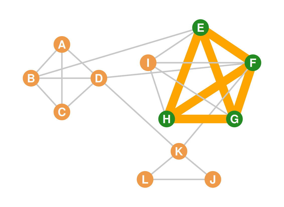
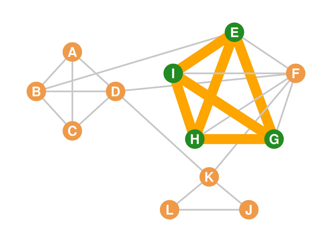
    • Clique of size 5
    • Clique of size 4
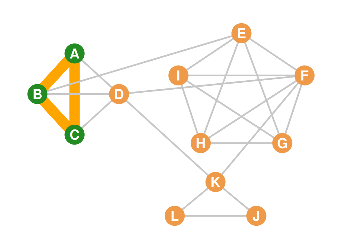
    • Clique of size 3

Cliques

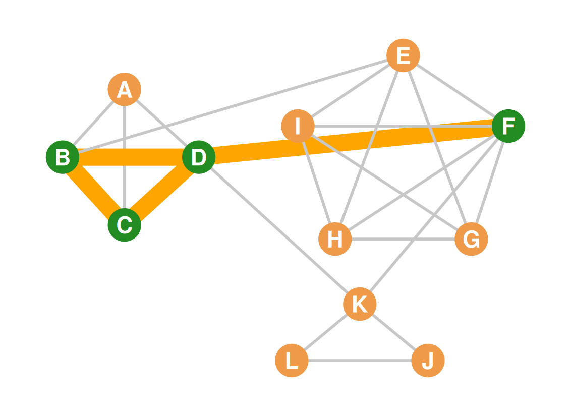
  • But three is the smallest a clique can be!
Cliques

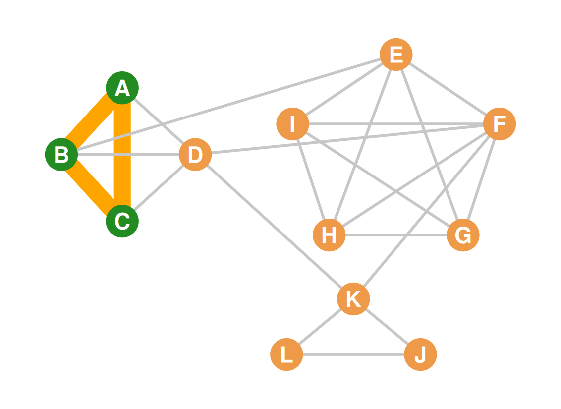
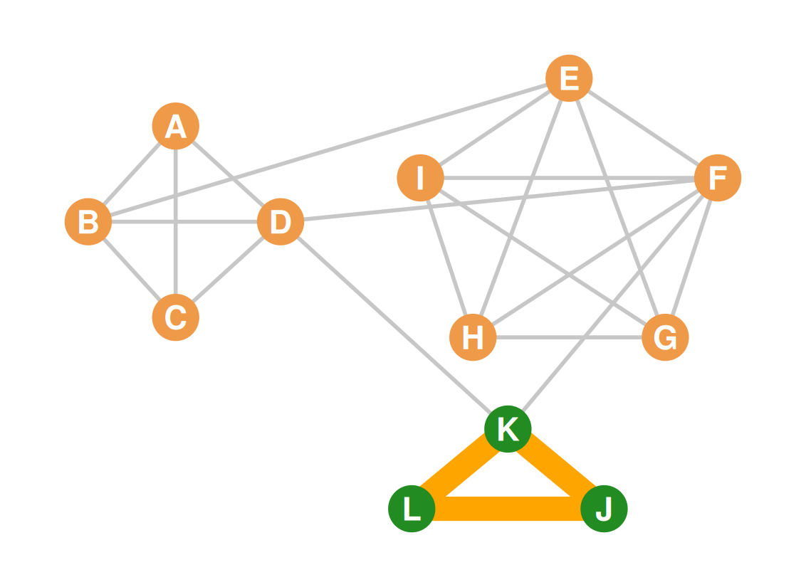
  • In an undirected graph the closed triad is a clique of size three!
    • This is a clique of size three!

Cliques

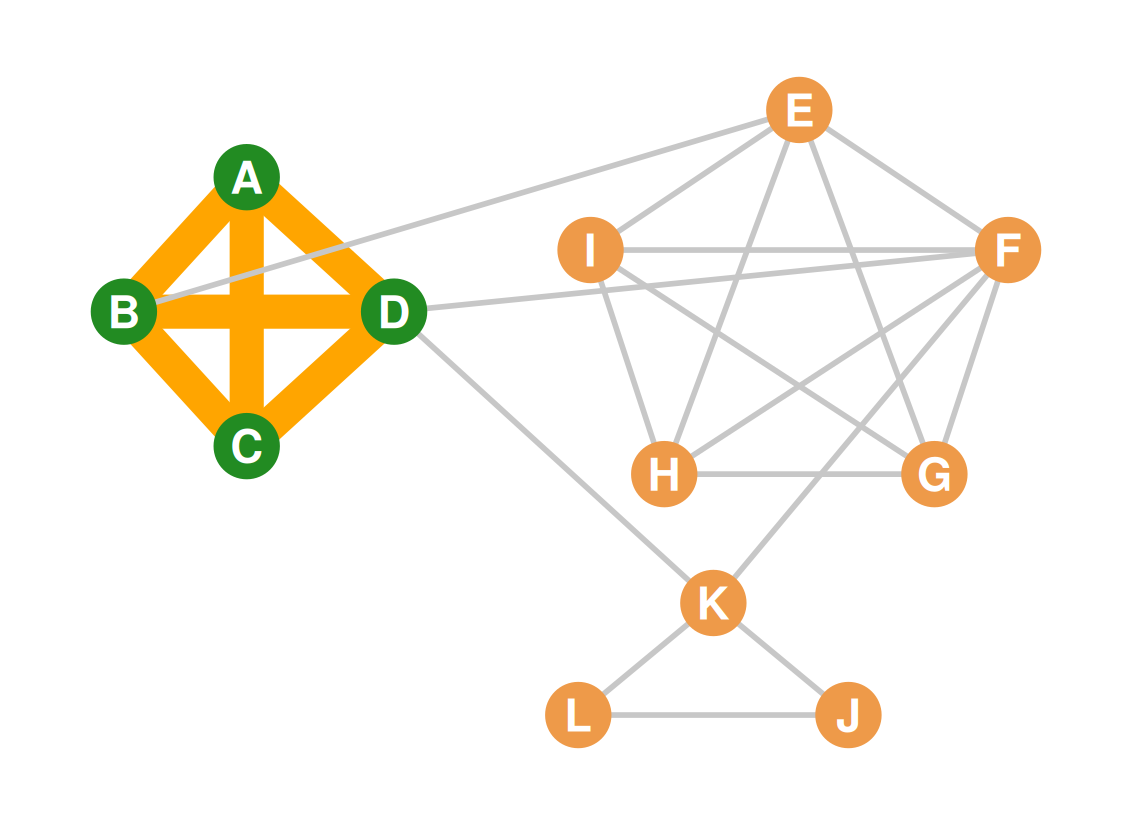
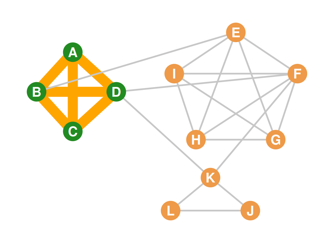
  • This is a clique of size 4!

Cliques

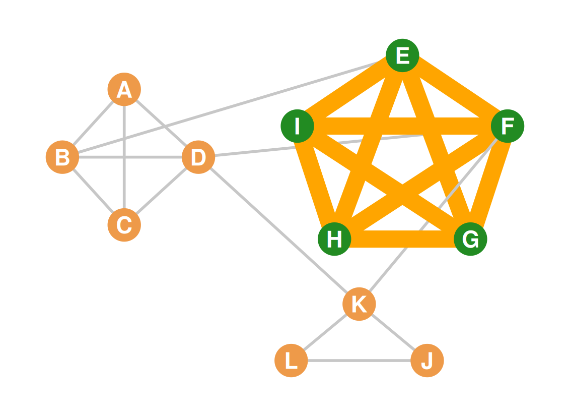
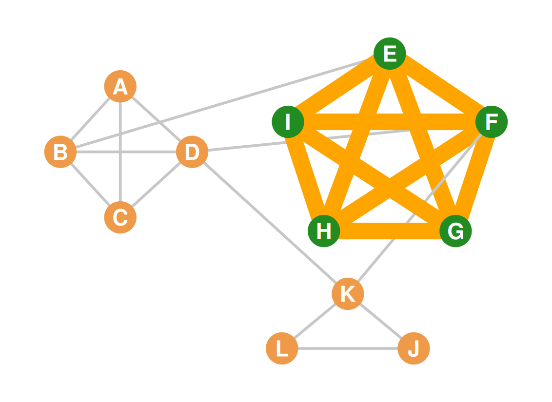
  • This is a clique of size 5!

Cliques

  • But three is the smallest a clique can be!
  • In an undirected graph the closed triad is a clique of size three!
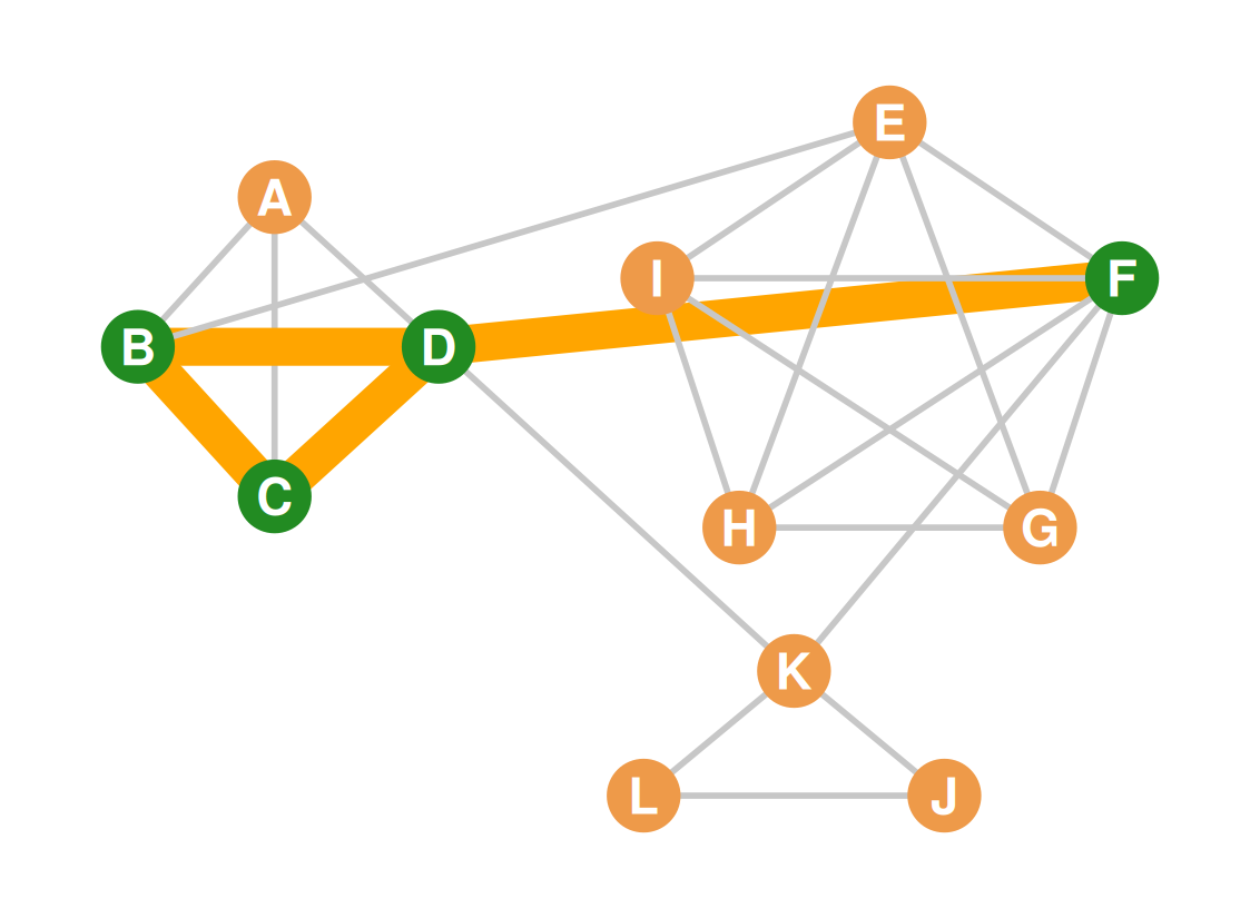
  • Is this subgraph a clique?

Cliques

  • No! It’s missing the \(BF\) edge

Cliques are referred to by their node set

  • Cliques are referred to by their node set
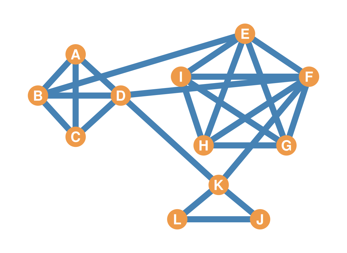
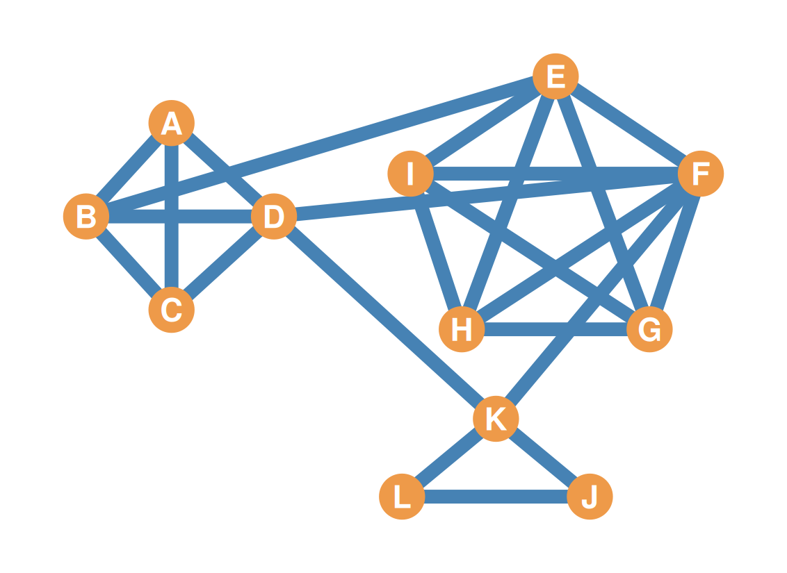
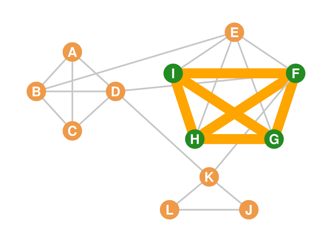
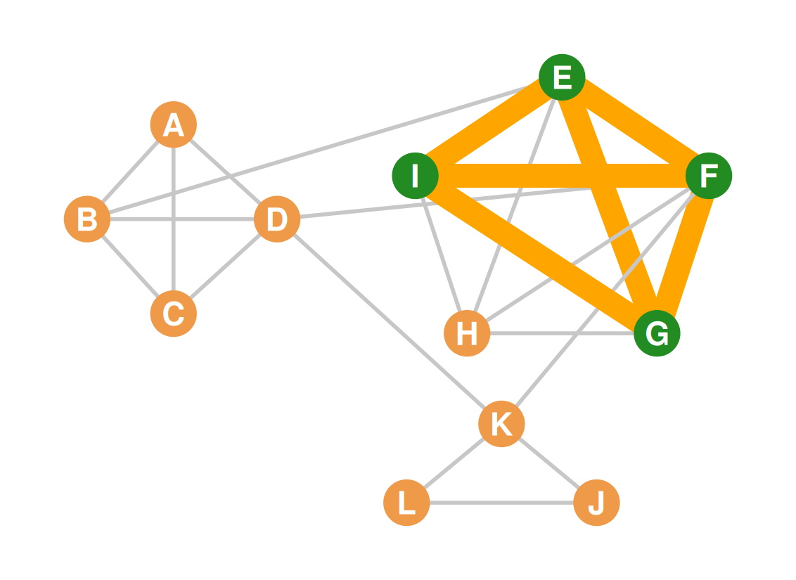
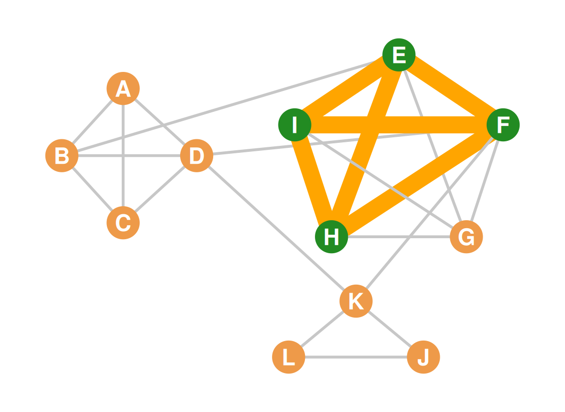
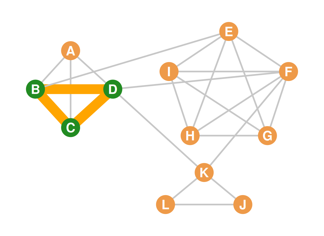
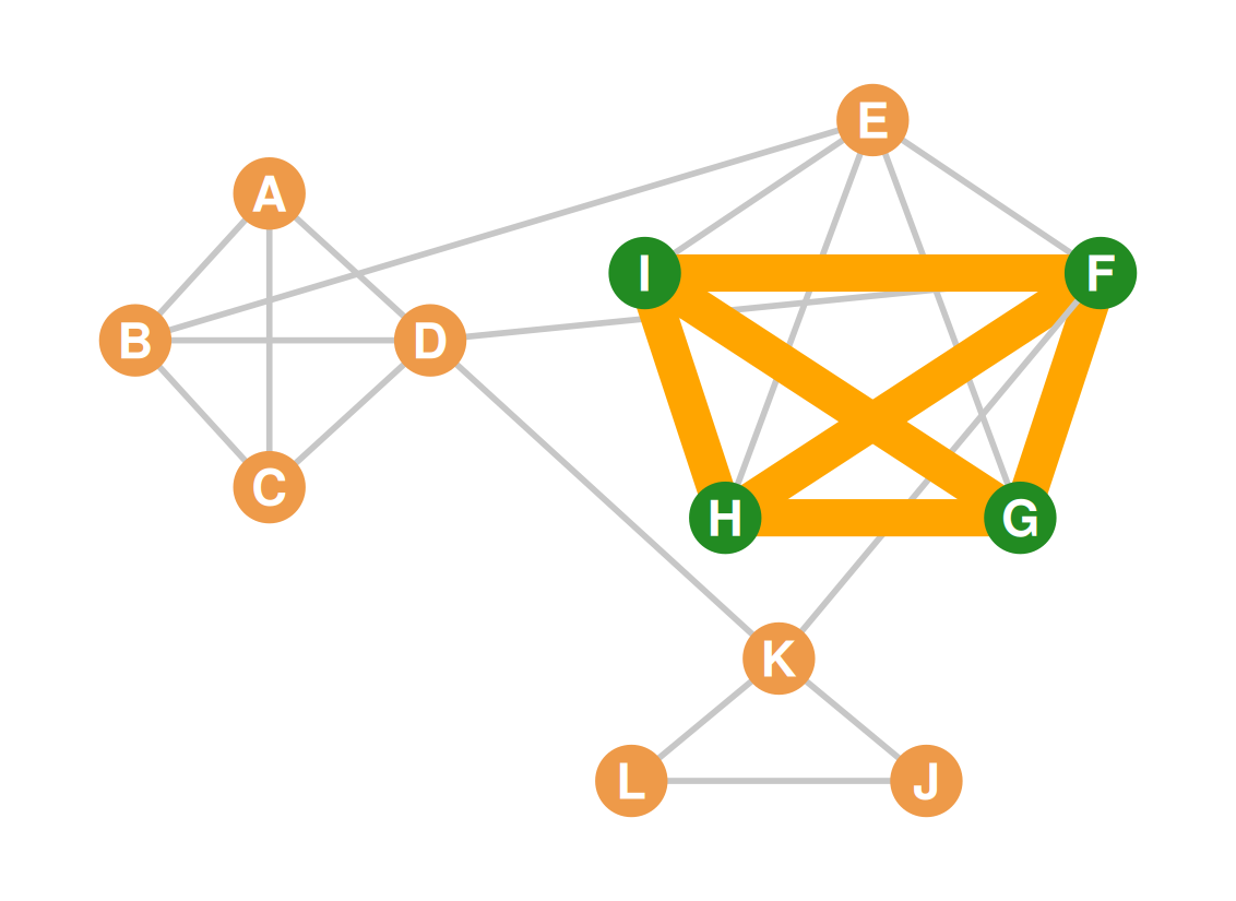
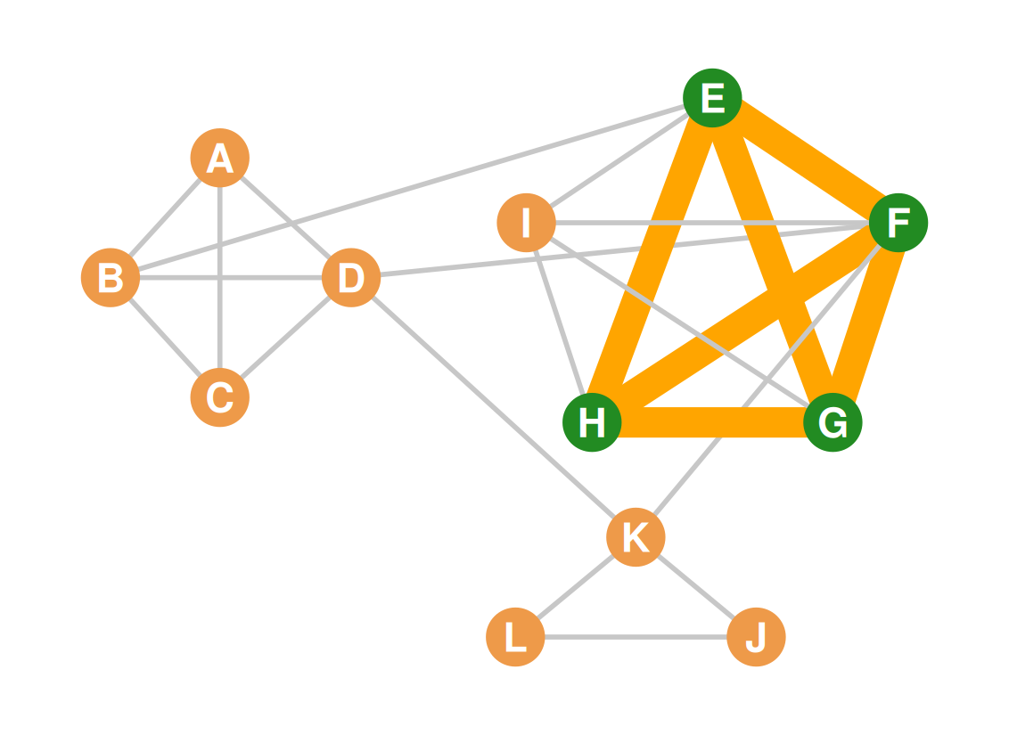
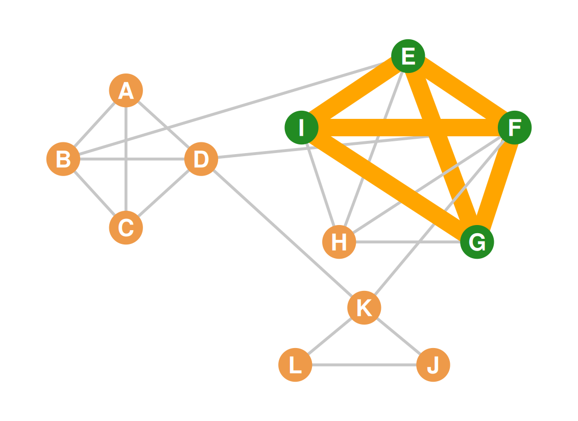
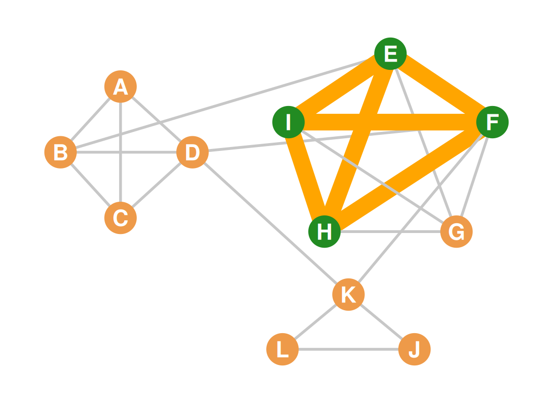
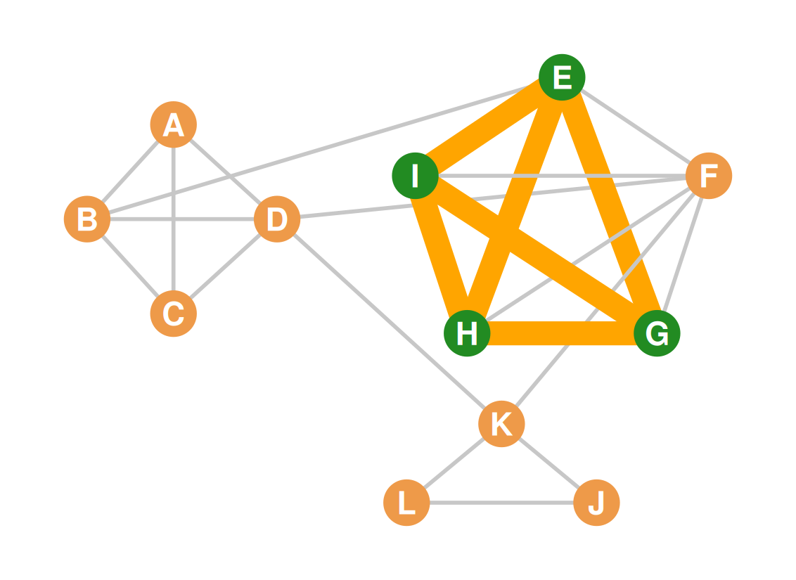
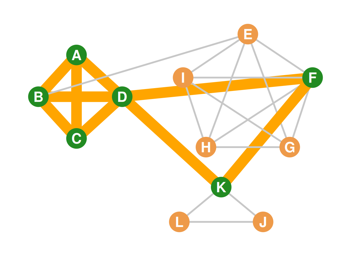
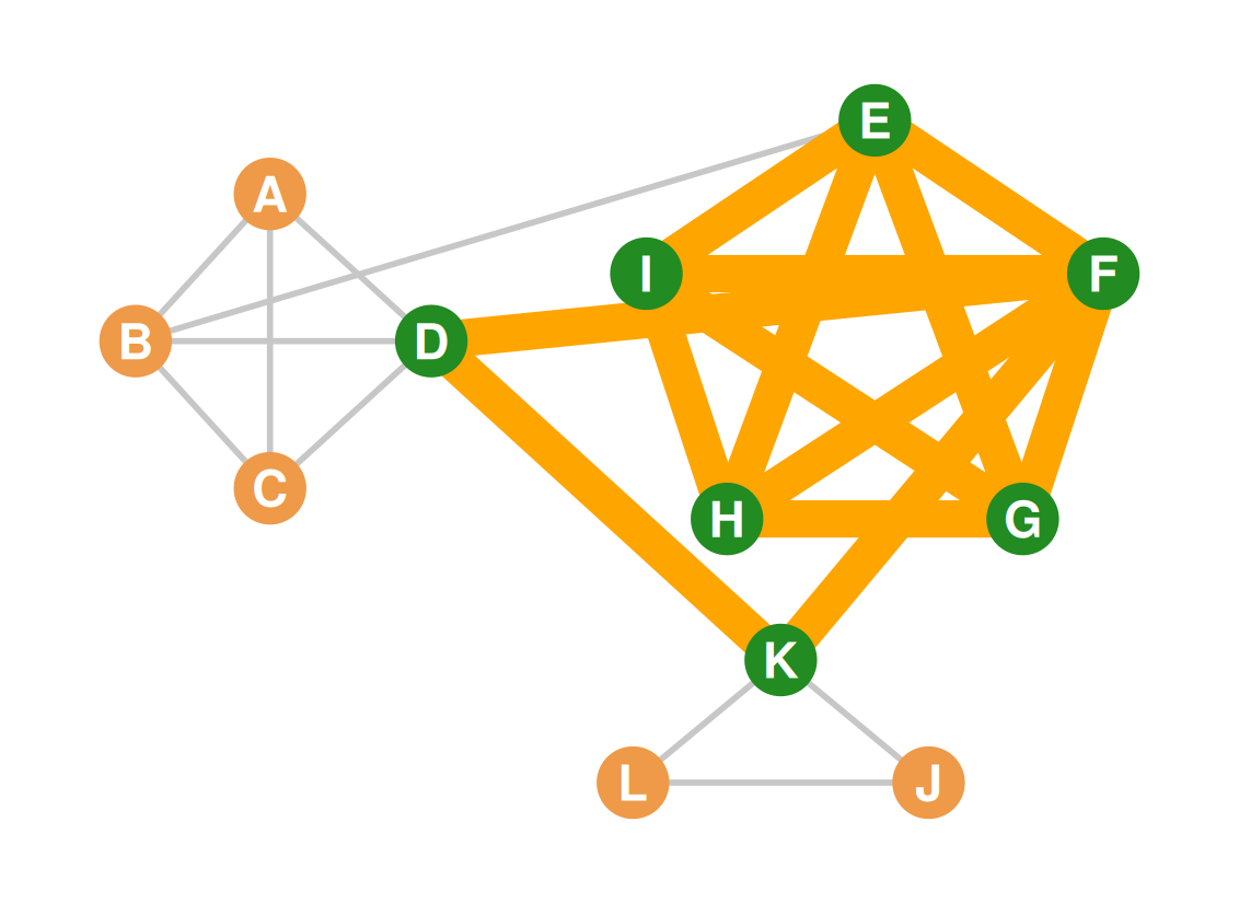
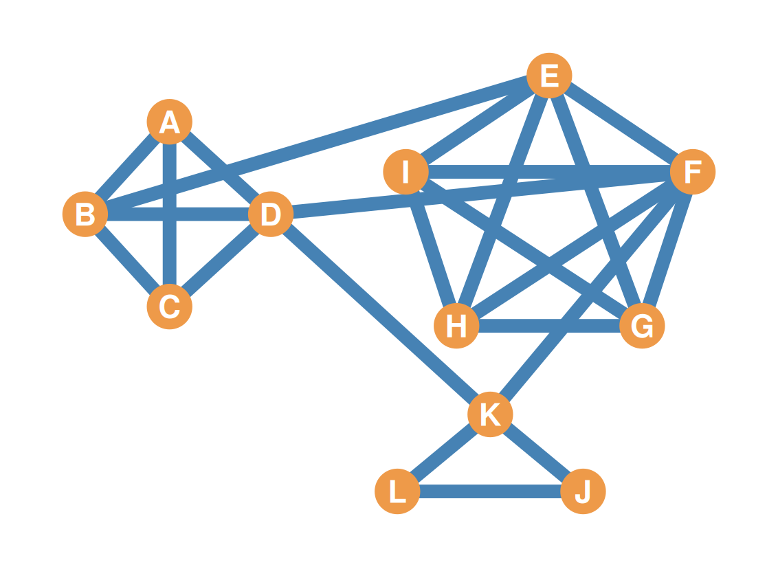
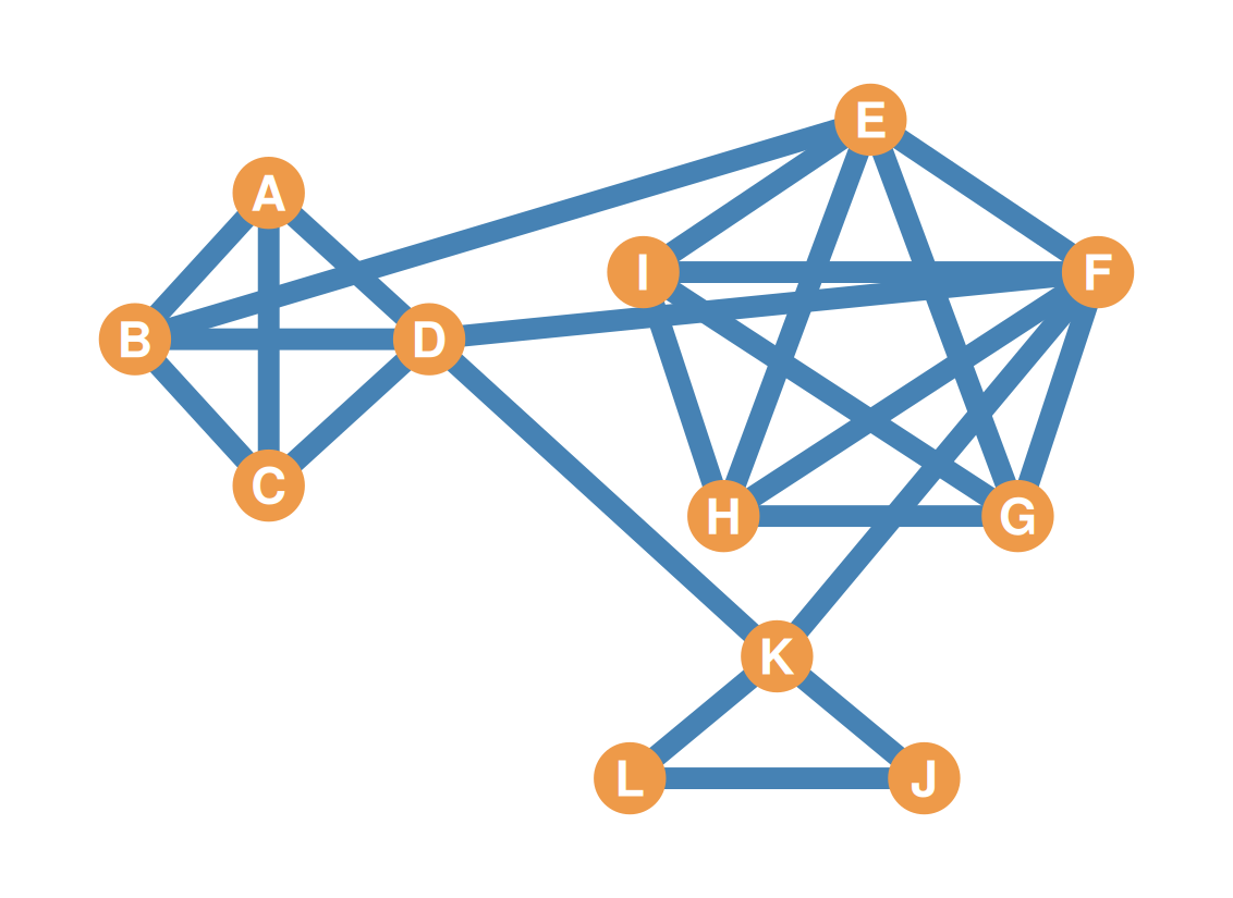
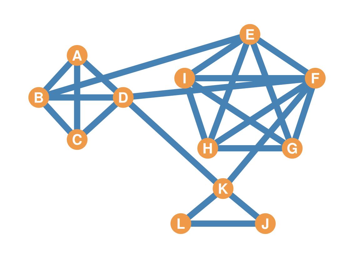
  • This graph has six cliques of size four:
    • \(\{A, B, C, D\}\)

Cliques are referred to by their node set

  • \(\{F, G, H, I\}\)

Cliques are referred to by their node set

  • \(\{E, F, G, H\}\)

Cliques are referred to by their node set

  • \(\{E, F, G, I\}\)

Cliques are referred to by their node set

  • \(\{E, F, H, I\}\)

Cliques are referred to by their node set

  • \(\{E, G, H, I\}\)
  • The node set of each clique has to be unique, but nodes can be shared!
Cliques can overlap: Nesting

  • Cliques can overlap for two reasons:
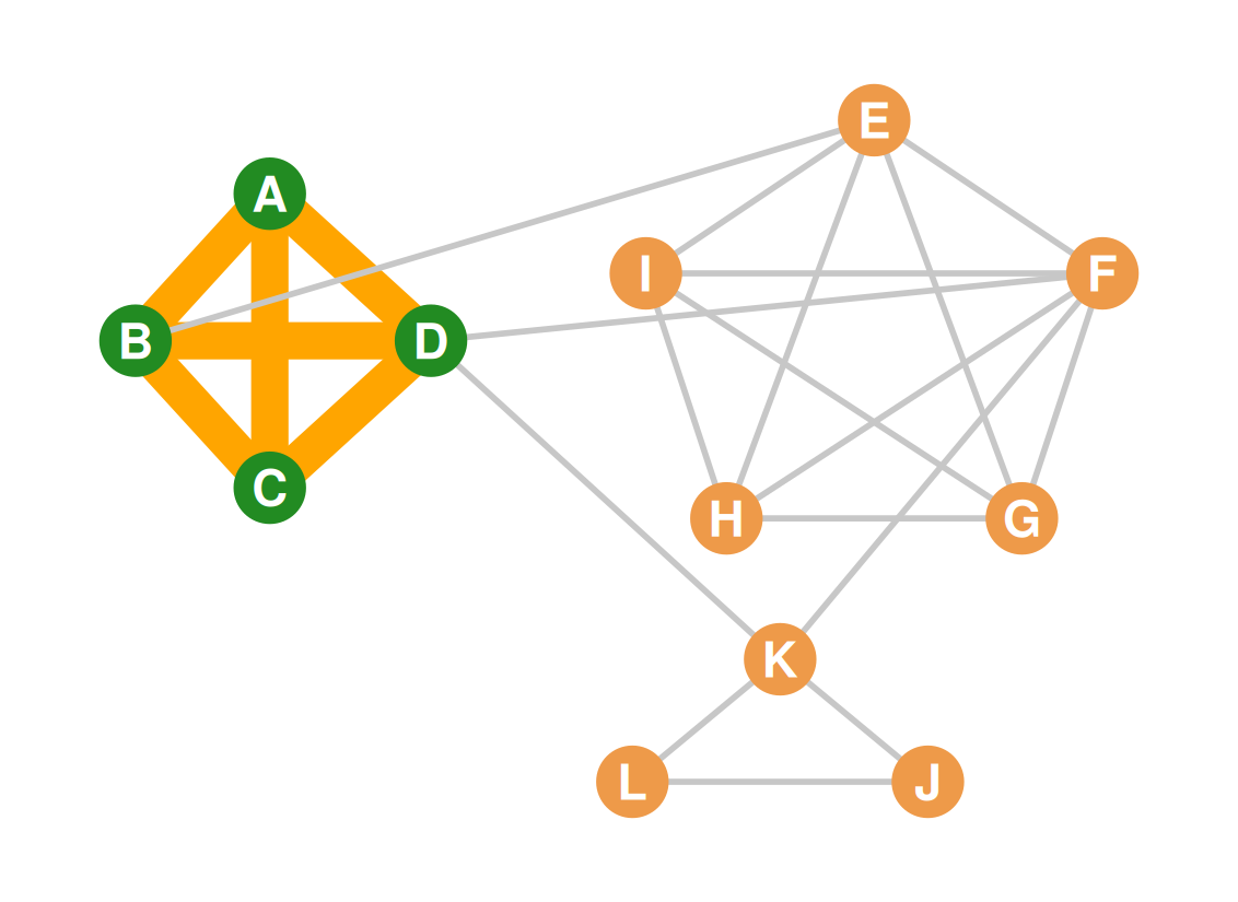
    • (1) Smaller cliques are nested within larger cliques
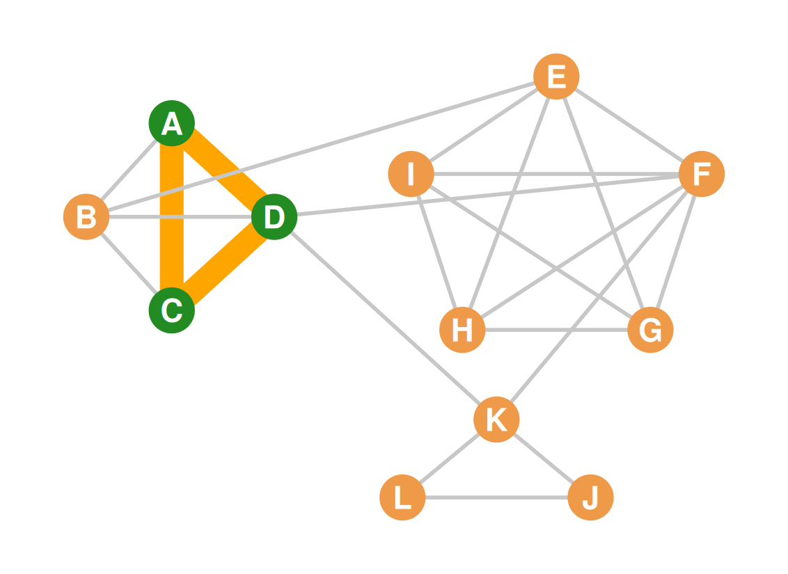
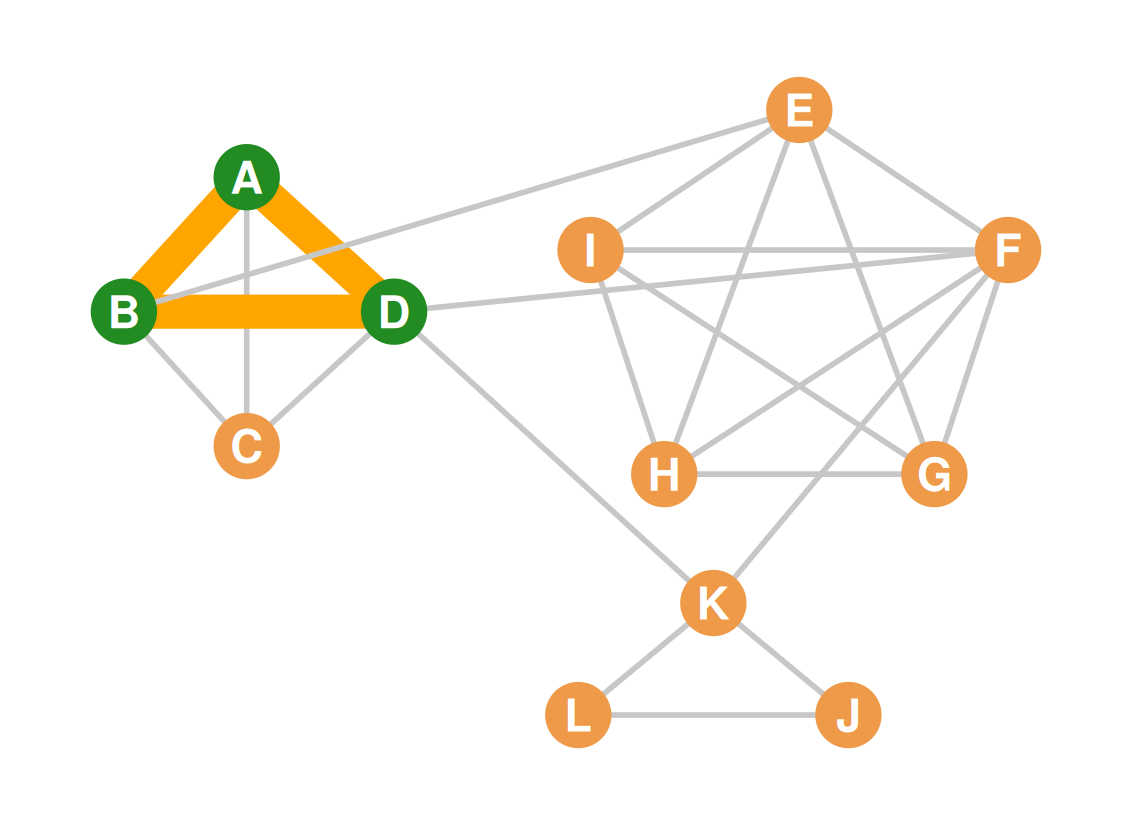
  • A clique of size four is made up of four cliques of size three!
Cliques can overlap: Nesting

  • \(\{A, B, C, D\}\)
  • \(\{A, B, C\}\)

Cliques can overlap: Nesting

  • \(\{B, C, D\}\)

Cliques can overlap: Nesting

  • \(\{A, C, D\}\)

Cliques can overlap: Nesting

  • \(\{A, B, D\}\)

Cliques can overlap: Nesting

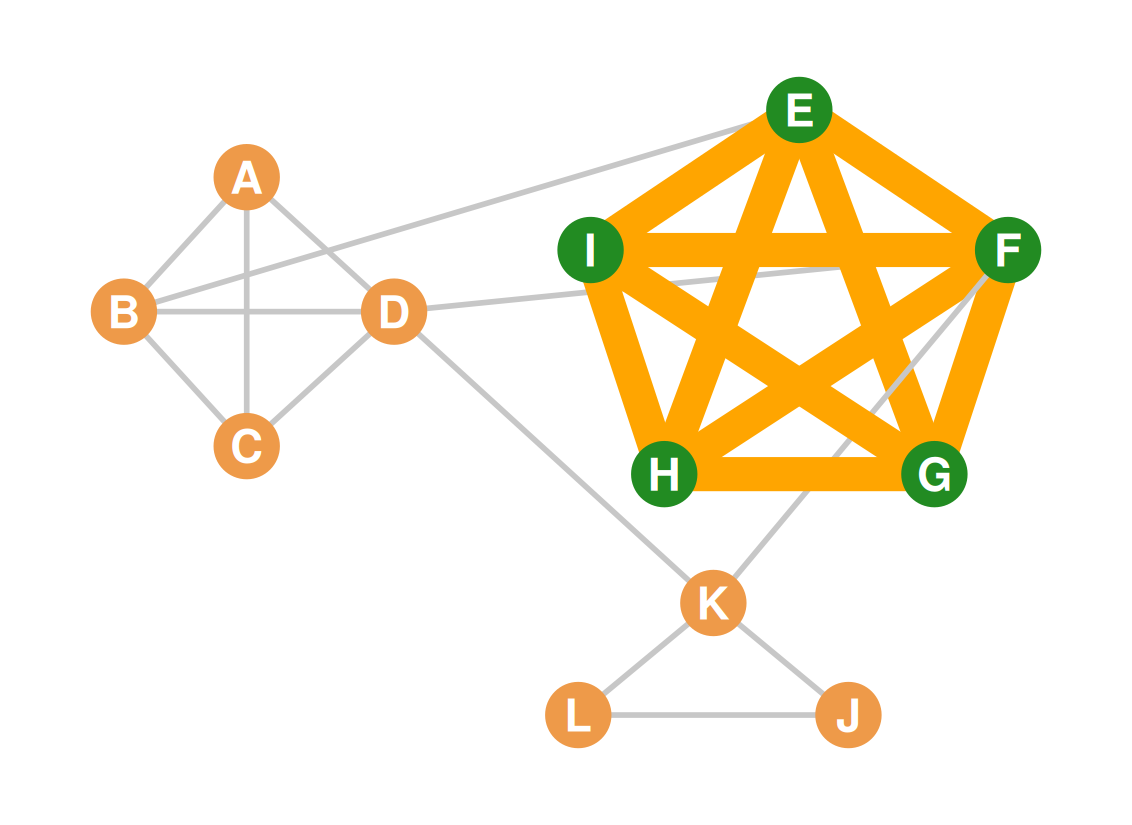
  • A clique of size five is made up of five cliques of size four!
Cliques can overlap: Nesting

  • \(\{E, F, G, H, I\}\)
  • \(\{F, G, H, I\}\)

Cliques can overlap: Nesting

  • \(\{E, F, G, H\}\)

Cliques can overlap: Nesting

  • \(\{E, F, G, I\}\)

Cliques can overlap: Nesting

  • \(\{E, F, H, I\}\)

Cliques can overlap: Nesting

  • \(\{E, G, H, I\}\)

Cliques can overlap: Shared members

  • Cliques can overlap for two reasons:
      1. Smaller cliques are nested within larger cliques
    • (2) Cliques can share members
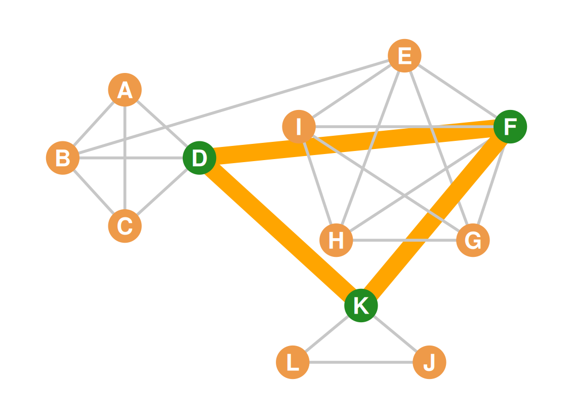
  • Node \(D\) is a member of both:
    • \(\{A, B, C, D\}\)
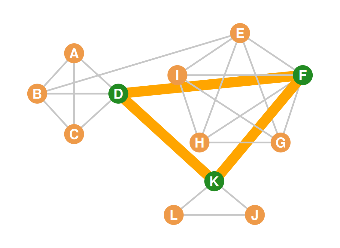
    • \(\{D, F, K\}\)

Cliques can overlap: Shared members

  • Node \(F\) is a member of both:
    • \(\{E, F, G, H, I\}\)
    • \(\{D, F, K\}\)

Cliques can overlap: Shared members

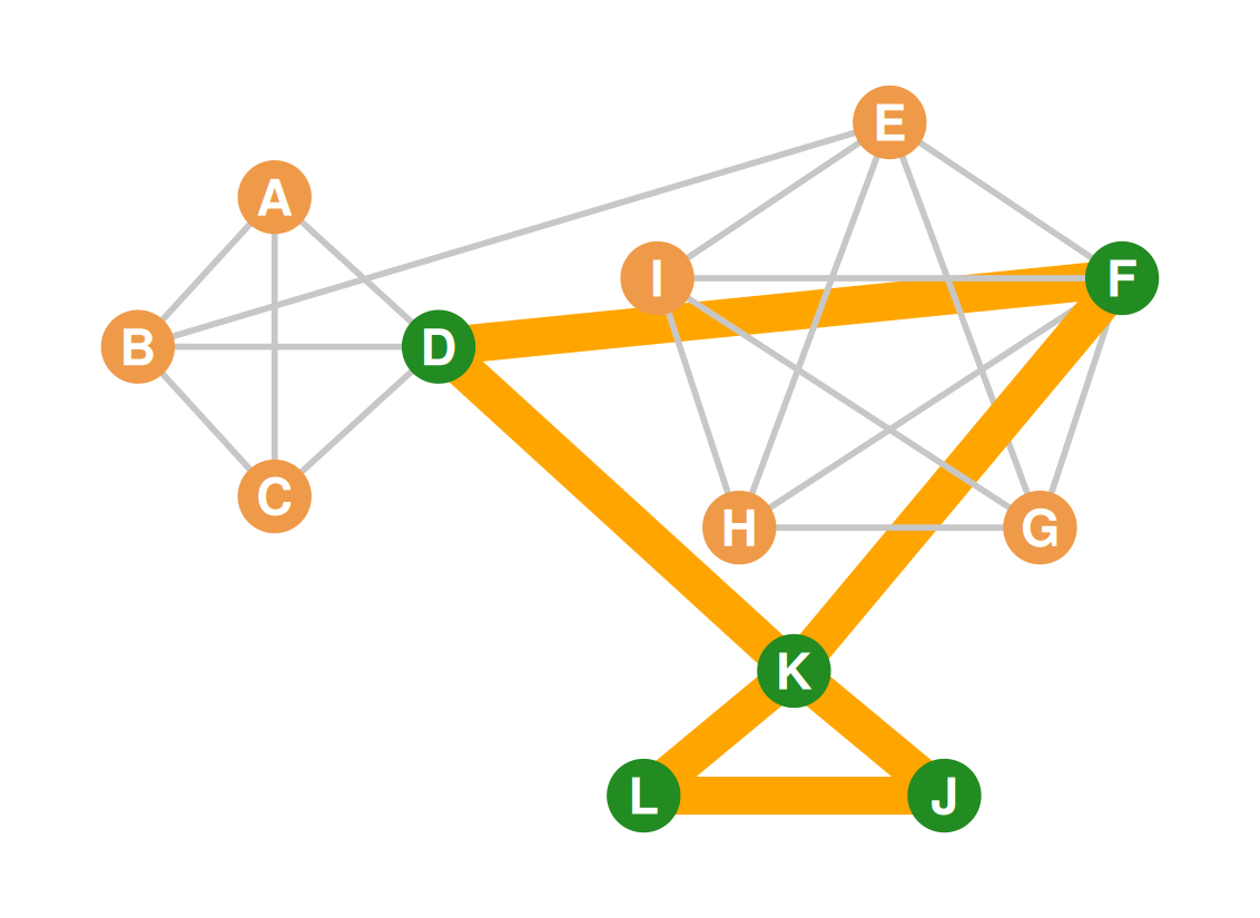
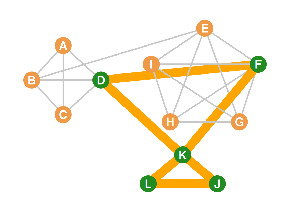
  • Node \(K\) is a member of both:
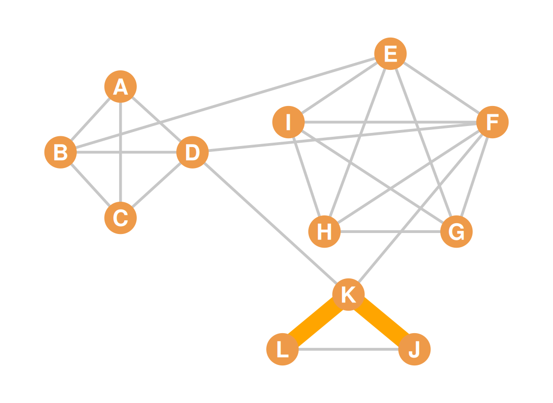
    • \(\{F, D, K\}\) and \(\{J, K, L\}\)

Cliques can overlap: Shared members

  • This means that the intersections of cliques are the members they share:
    • \(\{A, B, C, D\} \cap \{D, F, K\} = D\)
    • \(\{E, F, G, H, I\} \cap \{D, F, K\} = F\)
    • \(\{F, D, K\} \cap \{J, K, L\} = K\)

Cliques can overlap: Shared members

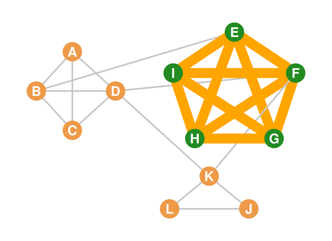
  • Cliques nested within other cliques share multiple members:
    • \(\{F, G, H, I\} \cap \{E, F, G, H\} = \{F, G, H\}\)
    • \(\{E, F, H, I\} \cap \{E, G, H, I\} = \{E, H, I\}\)
Part 3: Clique Analysis

Enumerating cliques in a network

  • In a graph we can enumerate all the cliques up to the maximum clique size
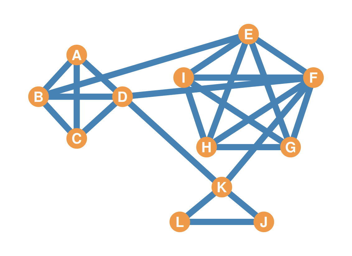
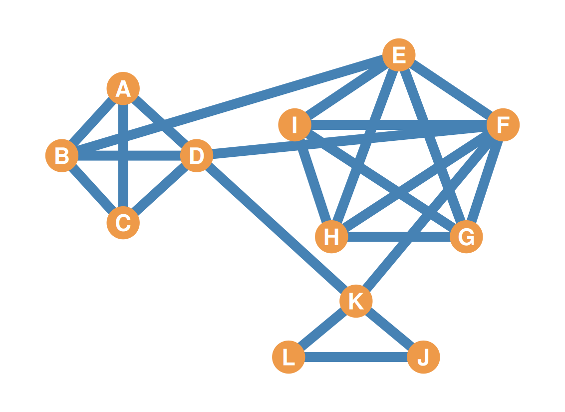
  • This graph has cliques of size three, four, and five. More specifically it has:
    • Sixteen cliques of size three
    • Six cliques of size four
    • One clique of size five
  • So \(16 + 6 + 1 = 23\) cliques total!
  • We can arrange this in a Person \(\times\) Clique affiliation matrix

The Clique Affiliation Matrix (\(C\))

C1 C2 C3 C4 C5 C6 C7 C8 C9 C10 C11 C12
A 0 0 1 0 0 0 0 1 1 1 0 0
B 0 0 1 0 0 0 0 1 1 0 1 0
C 0 0 1 0 0 0 0 1 0 1 1 0
D 0 0 1 0 0 0 0 0 1 1 1 1
E 1 0 0 1 1 1 1 0 0 0 0 0
F 1 1 0 1 1 1 0 0 0 0 0 1
G 1 1 0 1 1 0 1 0 0 0 0 0
H 1 1 0 1 0 1 1 0 0 0 0 0
I 1 1 0 0 1 1 1 0 0 0 0 0
J 0 0 0 0 0 0 0 0 0 0 0 0
K 0 0 0 0 0 0 0 0 0 0 0 1
L 0 0 0 0 0 0 0 0 0 0 0 0
C13 C14 C15 C16 C17 C18 C19 C20 C21 C22 C23
A 0 0 0 0 0 0 0 0 0 0 0
B 0 0 0 0 0 0 0 0 0 0 0
C 0 0 0 0 0 0 0 0 0 0 0
D 0 0 0 0 0 0 0 0 0 0 0
E 1 1 1 1 1 1 0 0 0 0 0
F 1 1 1 0 0 0 1 1 1 0 0
G 1 0 0 1 1 0 1 1 0 1 0
H 0 1 0 1 0 1 1 0 1 1 0
I 0 0 1 0 1 1 0 1 1 1 0
J 0 0 0 0 0 0 0 0 0 0 1
K 0 0 0 0 0 0 0 0 0 0 1
L 0 0 0 0 0 0 0 0 0 0 1
  • Rows are people; columns are the 23 cliques (\(C_1\) to \(C_{23}\)); a 1 marks membership.

The Clique Affiliation Matrix (\(C\))

C1 C2 C3 C4 C5 C6 C7 C8 C9 C10 C11 C12
A 0 0 1 0 0 0 0 1 1 1 0 0
B 0 0 1 0 0 0 0 1 1 0 1 0
C 0 0 1 0 0 0 0 1 0 1 1 0
D 0 0 1 0 0 0 0 0 1 1 1 1
E 1 0 0 1 1 1 1 0 0 0 0 0
F 1 1 0 1 1 1 0 0 0 0 0 1
G 1 1 0 1 1 0 1 0 0 0 0 0
H 1 1 0 1 0 1 1 0 0 0 0 0
I 1 1 0 0 1 1 1 0 0 0 0 0
J 0 0 0 0 0 0 0 0 0 0 0 0
K 0 0 0 0 0 0 0 0 0 0 0 1
L 0 0 0 0 0 0 0 0 0 0 0 0
Size 5 4 4 4 4 4 4 3 3 3 3 3
C13 C14 C15 C16 C17 C18 C19 C20 C21 C22 C23
A 0 0 0 0 0 0 0 0 0 0 0
B 0 0 0 0 0 0 0 0 0 0 0
C 0 0 0 0 0 0 0 0 0 0 0
D 0 0 0 0 0 0 0 0 0 0 0
E 1 1 1 1 1 1 0 0 0 0 0
F 1 1 1 0 0 0 1 1 1 0 0
G 1 0 0 1 1 0 1 1 0 1 0
H 0 1 0 1 0 1 1 0 1 1 0
I 0 0 1 0 1 1 0 1 1 1 0
J 0 0 0 0 0 0 0 0 0 0 1
K 0 0 0 0 0 0 0 0 0 0 1
L 0 0 0 0 0 0 0 0 0 0 1
Size 3 3 3 3 3 3 3 3 3 3 3
  • The column sums tell us the size of each clique!
  • We can tell which clique is which by looking at the members.

The Clique Affiliation Matrix (\(C\))

C1 C2 C3 C4 C5 C6 C7 C8 C9 C10 C11 C12 Cliques
A 0 0 1 0 0 0 0 1 1 1 0 0 4
B 0 0 1 0 0 0 0 1 1 0 1 0 4
C 0 0 1 0 0 0 0 1 0 1 1 0 4
D 0 0 1 0 0 0 0 0 1 1 1 1 5
E 1 0 0 1 1 1 1 0 0 0 0 0 11
F 1 1 0 1 1 1 0 0 0 0 0 1 12
G 1 1 0 1 1 0 1 0 0 0 0 0 11
H 1 1 0 1 0 1 1 0 0 0 0 0 11
I 1 1 0 0 1 1 1 0 0 0 0 0 11
J 0 0 0 0 0 0 0 0 0 0 0 0 1
K 0 0 0 0 0 0 0 0 0 0 0 1 2
L 0 0 0 0 0 0 0 0 0 0 0 0 1
C13 C14 C15 C16 C17 C18 C19 C20 C21 C22 C23 Cliques
A 0 0 0 0 0 0 0 0 0 0 0 4
B 0 0 0 0 0 0 0 0 0 0 0 4
C 0 0 0 0 0 0 0 0 0 0 0 4
D 0 0 0 0 0 0 0 0 0 0 0 5
E 1 1 1 1 1 1 0 0 0 0 0 11
F 1 1 1 0 0 0 1 1 1 0 0 12
G 1 0 0 1 1 0 1 1 0 1 0 11
H 0 1 0 1 0 1 1 0 1 1 0 11
I 0 0 1 0 1 1 0 1 1 1 0 11
J 0 0 0 0 0 0 0 0 0 0 1 1
K 0 0 0 0 0 0 0 0 0 0 1 2
L 0 0 0 0 0 0 0 0 0 0 1 1
  • The row sums give the number of cliques each person belongs to!

Clique membership as a centrality metric

  • The rank order of the number of cliques a node belongs to is a centrality metric on the nodes!
    • \(F\) (12 cliques) seems to be in the middle of everything!
    • \(E\), \(G\), \(H\), \(I\), \(D\) are also central
    • But mainly because they belong to a large clique
    • \(J\) and \(L\) are the least central: they belong to one small clique
Node Cliques
F 12
E 11
G 11
H 11
I 11
D 5
A 4
B 4
C 4
K 2
J 1
L 1

Restricting to the large cliques

C1 C2 C3 C4 C5 C6 C7 Cliques
A 0 0 1 0 0 0 0 1
B 0 0 1 0 0 0 0 1
C 0 0 1 0 0 0 0 1
D 0 0 1 0 0 0 0 1
E 1 0 0 1 1 1 1 5
F 1 1 0 1 1 1 0 5
G 1 1 0 1 1 0 1 5
H 1 1 0 1 0 1 1 5
I 1 1 0 0 1 1 1 5
J 0 0 0 0 0 0 0 0
K 0 0 0 0 0 0 0 0
L 0 0 0 0 0 0 0 0
  • Let’s just restrict ourselves to the large cliques (the one clique of size 5 and the six cliques of size 4)!
  • We have some isolates!
    • \(j\), \(k\), and \(l\) belong to no large clique

Restricting to the large cliques

C1 C2 C3 C4 C5 C6 C7
A 0 0 1 0 0 0 0
B 0 0 1 0 0 0 0
C 0 0 1 0 0 0 0
D 0 0 1 0 0 0 0
E 1 0 0 1 1 1 1
F 1 1 0 1 1 1 0
G 1 1 0 1 1 0 1
H 1 1 0 1 0 1 1
I 1 1 0 0 1 1 1
Size 5 4 4 4 4 4 4
  • Let’s just restrict ourselves to the large cliques
  • Let’s get rid of the isolates!

The Clique Overlap Matrix (\(O\))

C1 C2 C3 C4 C5 C6 C7
C1 5 4 0 4 4 4 4
C2 4 4 0 3 3 3 3
C3 0 0 4 0 0 0 0
C4 4 3 0 4 3 3 3
C5 4 3 0 3 4 3 3
C6 4 3 0 3 3 4 3
C7 4 3 0 3 3 3 4
  • \(O = C^T C\): the clique overlap matrix
  • The diagonal cells are the size of each clique!
  • The off-diagonal cells are the number of people the row clique has in common with the column clique!

The Clique Overlap Matrix (\(O\))

C1 C2 C3 C4 C5 C6 C7
C1 -- 4 0 4 4 4 4
C2 4 -- 0 3 3 3 3
C3 0 0 -- 0 0 0 0
C4 4 3 0 -- 3 3 3
C5 4 3 0 3 -- 3 3
C6 4 3 0 3 3 -- 3
C7 4 3 0 3 3 3 --
  • The diagonal is the size of each clique
  • The off-diagonals are the number of people the row clique has in common with the column clique!
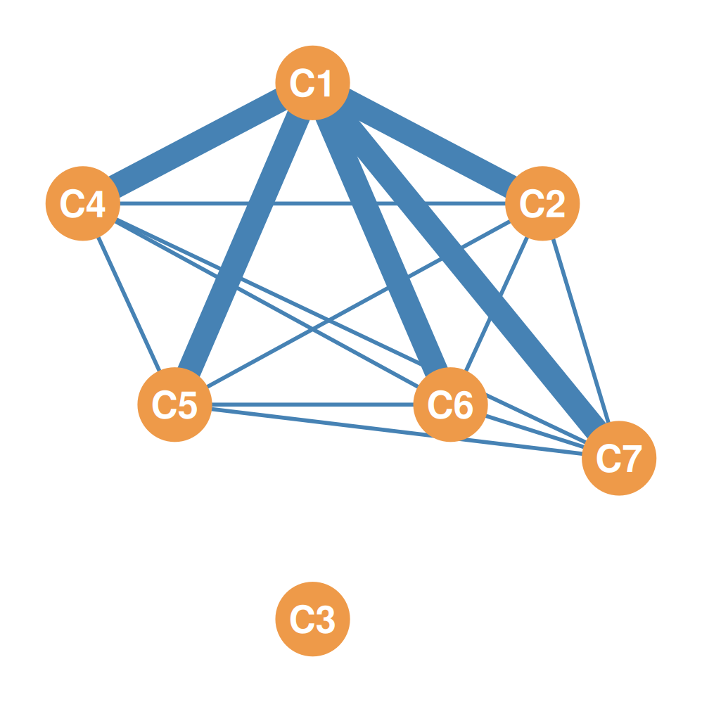
  • \(C_3\) (the \(\{A, B, C, D\}\) clique) is an isolate in the overlap matrix: it does not share members with any other large clique

The Clique Graph

  • We can represent the clique overlap matrix using the weighted clique graph!
  • A weighted network where:
    • Nodes are cliques (\(C_1\) to \(C_7\))
    • Edges are weighted by the number of shared members
  • \(C_3\) appears as an isolate in the clique graph: it shares no members with the other large cliques
We can analyze \(C\) like any two-mode network

  • We can analyze the structure of the clique affiliation matrix the same way we analyze any two-mode network!
  • The \(C\) matrix is a person-by-group affiliation network (Breiger, 1974):
    • \(CC^T\) gives the person co-membership matrix (number of cliques shared by each pair of people)
    • \(C^TC\) gives the clique overlap matrix (number of people shared by each pair of cliques)
  • This connects subgroup analysis directly to the affiliation networks toolbox.

Part 4: N-Cliques

N-Cliques

  • Some subgraphs are not complete graphs (cliques) but they are almost there
  • They are quasi-groups
  • We can relax the strict clique definition to accommodate!

N-Cliques

  • Some subgraphs are not complete graphs (cliques) but they are almost there
  • They are quasi-groups
  • We can relax the strict clique definition to accommodate!
  • An \(n\)-clique is a maximal subgraph in which each node can reach every other node in at most \(n\) steps:
    • \[d(u, v) \le n \quad \text{for all } u, v \in V'\]
    • 2-clique, 3-clique, 4-clique, etc.

A 2-clique of order 7

  • The seven-node subgraph on the right is a 2-clique of order 7!
  • Every pair of nodes can reach every other node in at most 2 steps
  • The geodesic distance matrix (computed on the whole graph) confirms it: the largest entry among these nodes is 2
A B C D E F K
A -- 1 1 1 2 2 2
B 1 -- 1 1 1 2 2
C 1 1 -- 1 2 2 2
D 1 1 1 -- 2 1 1
E 2 1 2 2 -- 1 2
F 2 2 2 1 1 -- 1
K 2 2 2 1 2 1 --

Adding a node breaks the 2-clique

  • Add node \(J\) to the subgraph
  • \(d(A, J) = 3\): the 2-clique property fails!
  • No longer a 2-clique!
A B C D E F K J
A -- 1 1 1 2 2 2 3
B 1 -- 1 1 1 2 2 3
C 1 1 -- 1 2 2 2 3
D 1 1 1 -- 2 1 1 2
E 2 1 2 2 -- 1 2 3
F 2 2 2 1 1 -- 1 2
K 2 2 2 1 2 1 -- 1
J 3 3 3 2 3 2 1 --

Adding another node: still no 2-clique

  • Add node \(G\) instead of \(J\)
  • \(d(A, G) = 3\): still no 2-clique!
A B C D E F K G
A -- 1 1 1 2 2 2 3
B 1 -- 1 1 1 2 2 2
C 1 1 -- 1 2 2 2 3
D 1 1 1 -- 2 1 1 2
E 2 1 2 2 -- 1 2 1
F 2 2 2 1 1 -- 1 1
K 2 2 2 1 2 1 -- 2
G 3 2 3 2 1 1 2 --

The whole graph is a 3-clique

  • Take all twelve nodes
  • The largest geodesic distance in the whole graph is 3 (for example, \(d(A, J) = 3\))
  • So the whole graph is a 3-clique!

Part 5: Graph Connectivity

Graph connectivity: Components

  • A graph is connected if there exists a (finite) path between each pair of nodes
  • A graph is disconnected if there does not exist a path connecting every pair of nodes
  • A connected subgraph is called a component
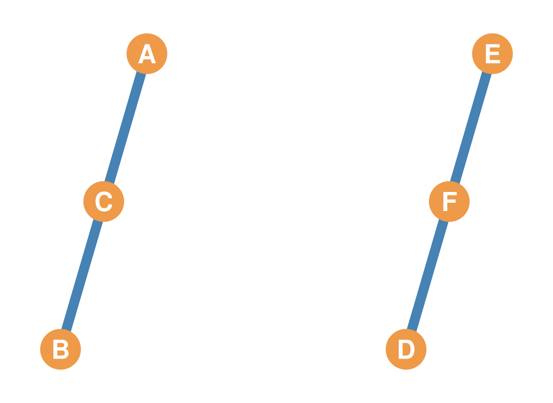
  • These are two different components

Graph connectivity: Components

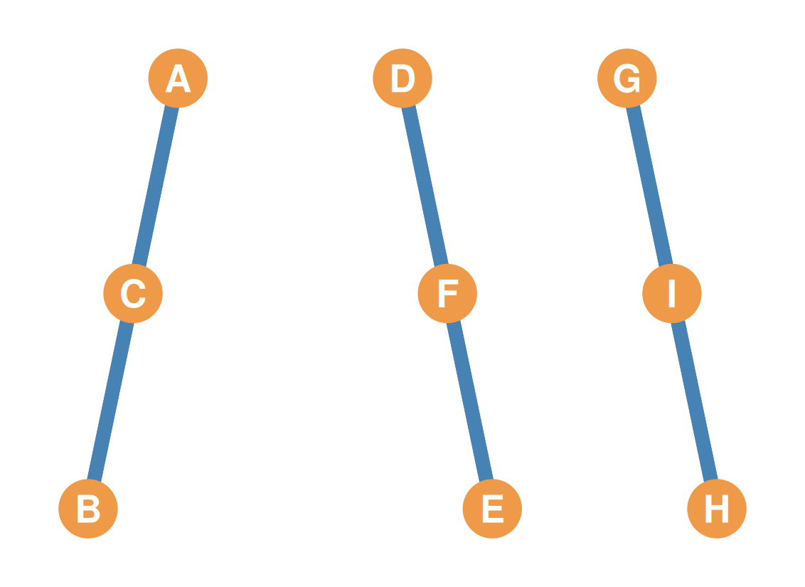
  • If a graph has more than one component it is by definition disconnected
  • These are three different components

The giant component

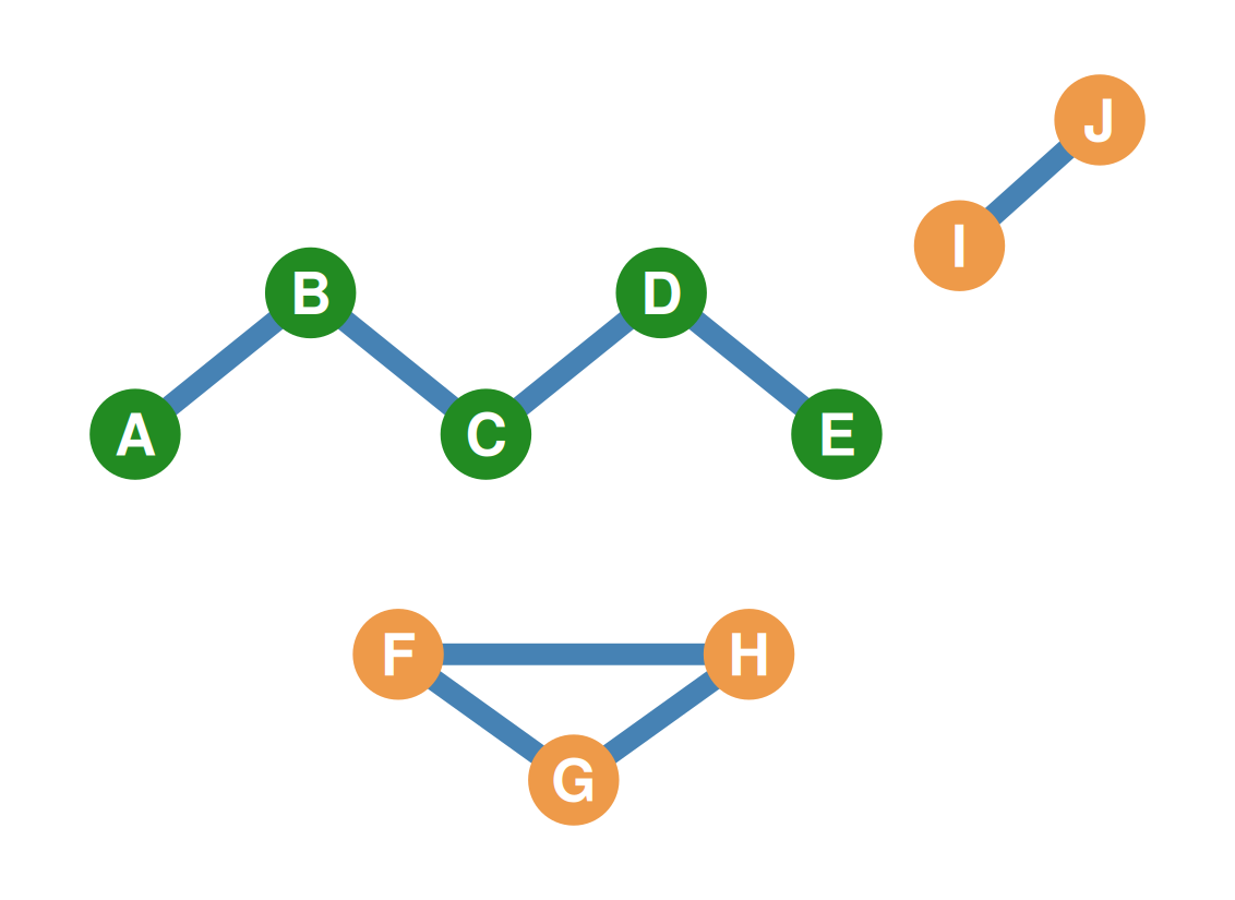
  • The connected subgraph containing the largest number of vertices in a graph is called the giant component
  • This is the giant component!

Graph connectivity: K-Connectivity

  • We can disconnect a graph by removing edges
  • We can also disconnect a graph by removing nodes
  • It can be easier to disconnect a graph by removing nodes, because nodes take their links with them!
Graph connectivity: K-Connectivity

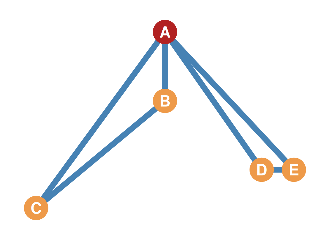
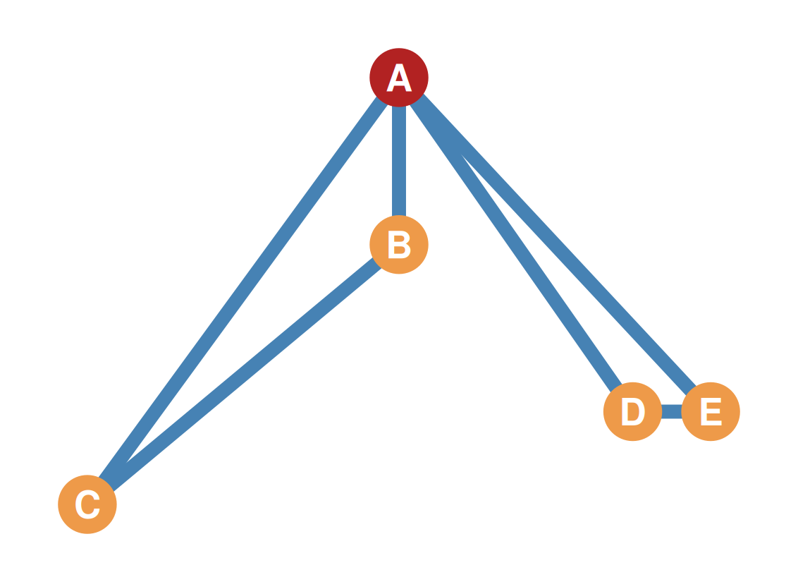
  • The \(k\)-connectivity of a graph is the minimum number of nodes we need to remove to disconnect it
  • Here \(k\)-connectivity = 1
  • Some nodes are more “important” because they serve as the connectors
  • Can you guess what kind of centrality “connector” nodes are more likely to have?
Graph connectivity: K-Connectivity

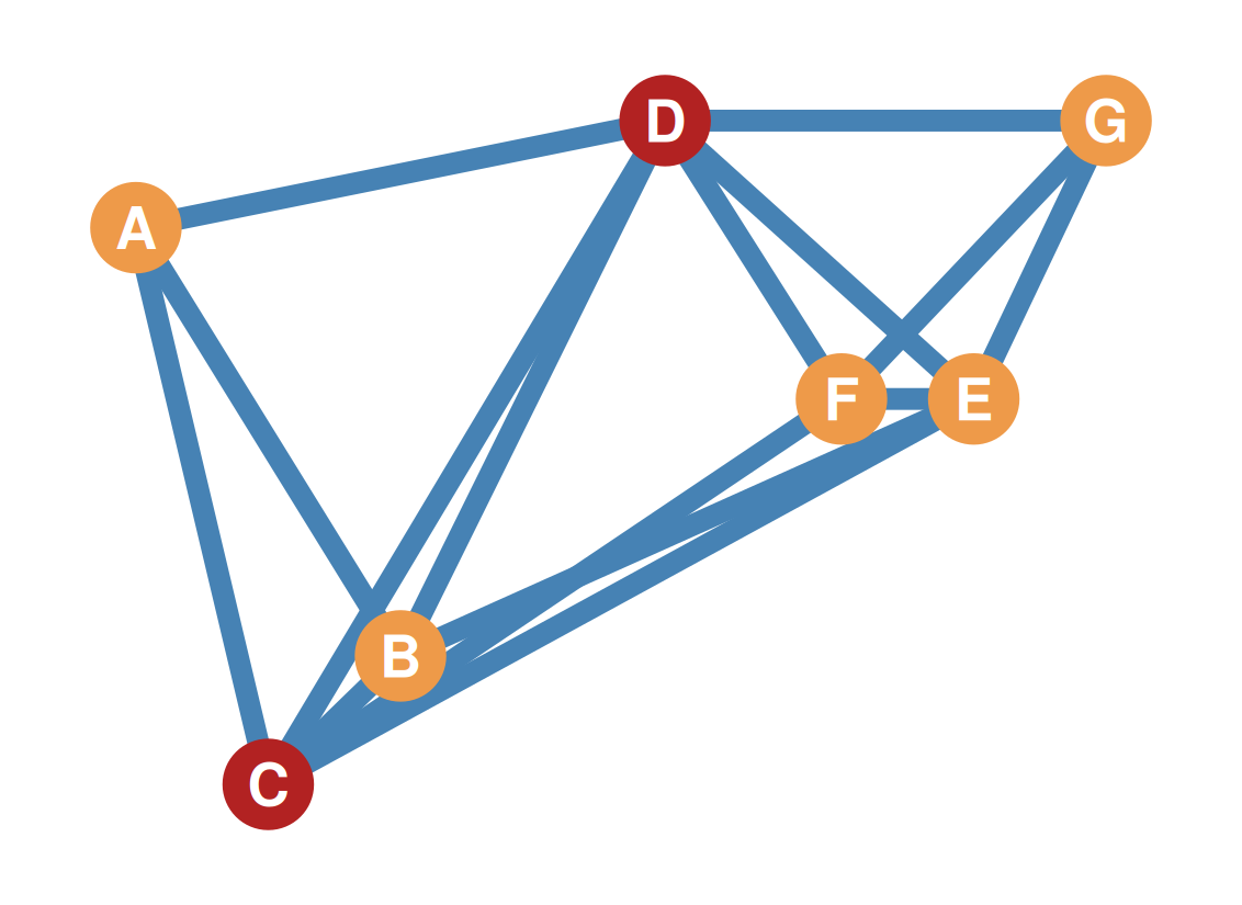
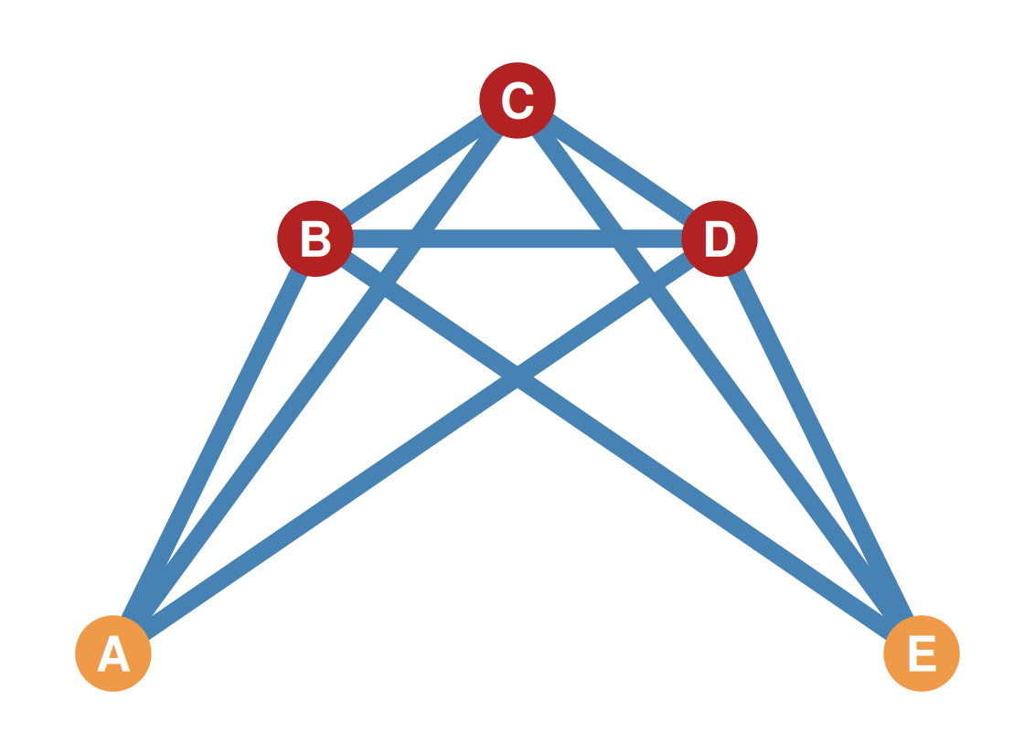
  • The better connected the structure, the more nodes we need to remove to disconnect it
  • Here \(k\)-connectivity = 2: remove the two shared nodes…
Graph connectivity: K-Connectivity

  • Here \(k\)-connectivity = 3: removing two nodes is not enough!
Edge Connectivity

  • Some graphs are easy to disconnect by removing edges (only a few links required)
  • Others are hard to disconnect (many links must go)
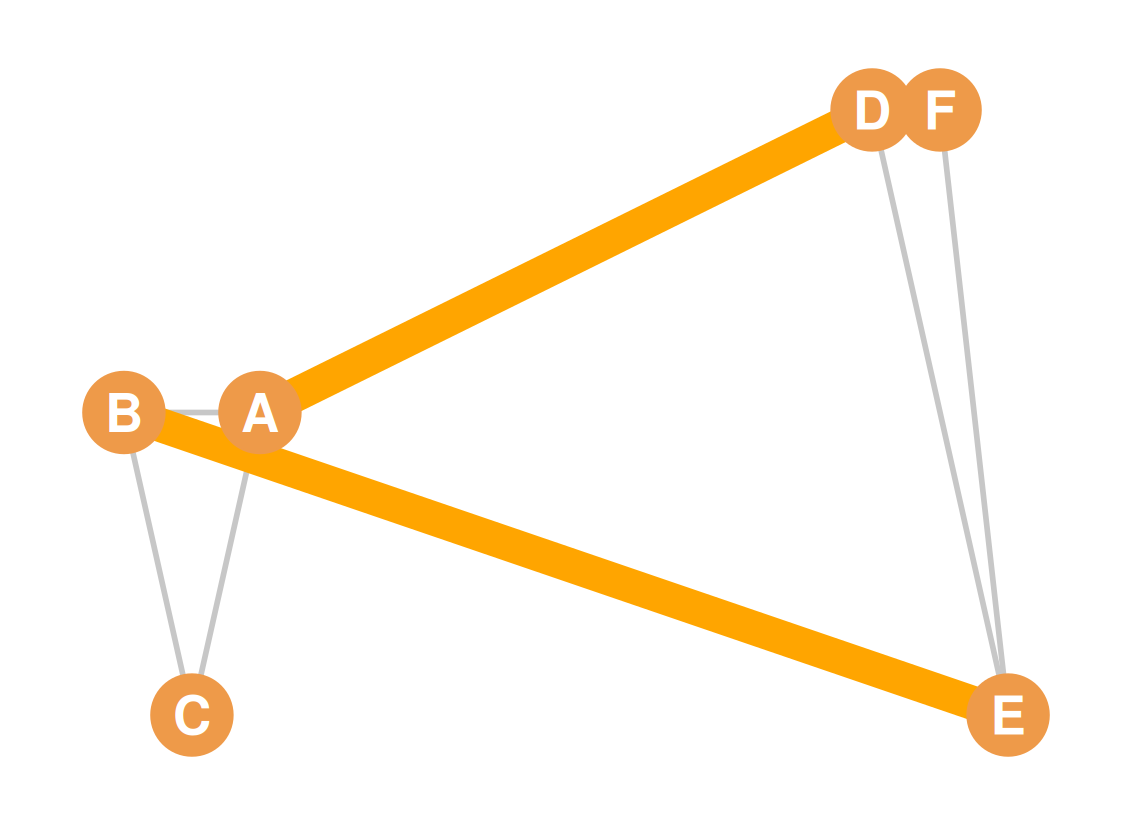
  • The edge-connectivity of a graph is the minimum number of edges that must be removed to disconnect the graph
  • Here edge connectivity = 2: remove the two links and it is disconnected!
Bridges

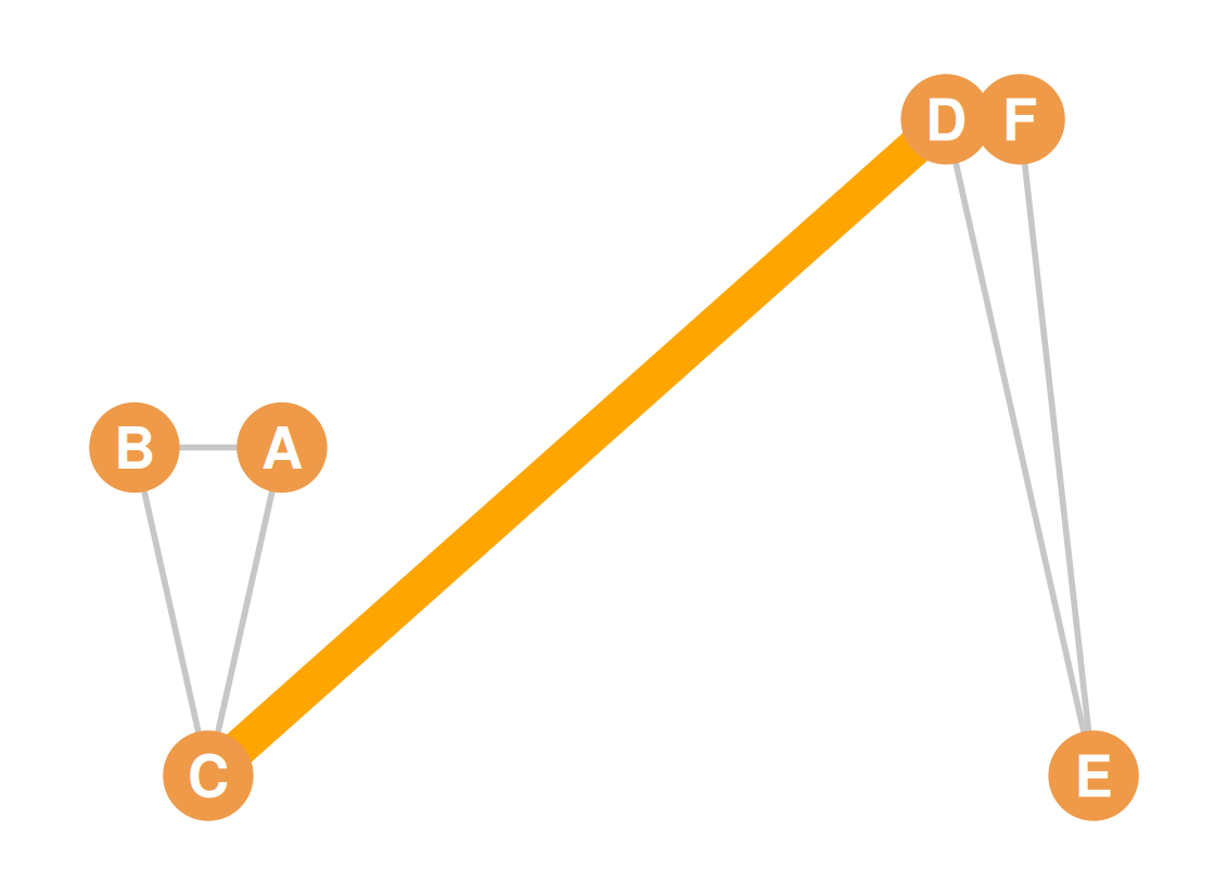
  • Graphs with edge connectivity equal to one have a special edge
  • This edge is called a bridge
  • Here edge connectivity = 1: this edge is a bridge!
Articulation nodes

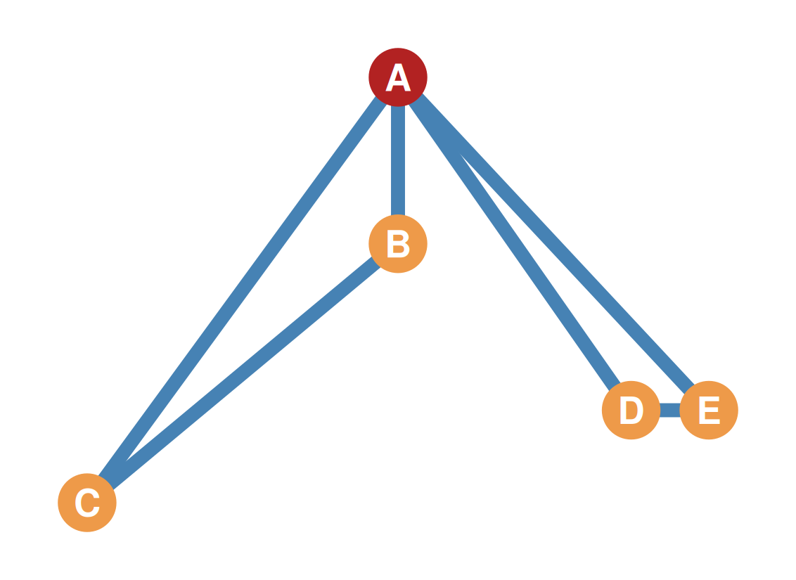
  • The \(k\)-connectivity of a graph is the minimum number of nodes that must be removed to disconnect the graph
  • Graphs with \(k\)-connectivity equal to one have a special node
  • This node is called an articulation node
  • Here \(k\)-connectivity = 1: this is an articulation node!
Node and edge connectivity differ

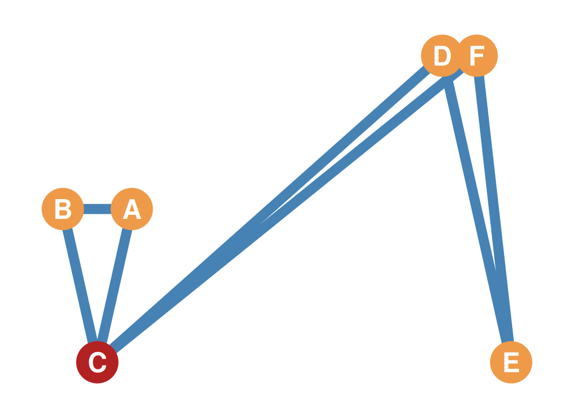
  • The \(k\)-connectivity and edge connectivity of a graph do not have to be the same number!
  • The \(k\)-connectivity of this graph is 1: it has an articulation node
Node and edge connectivity differ

  • But the edge connectivity is 2!
  • We need to remove a minimum of two edges to disconnect this graph
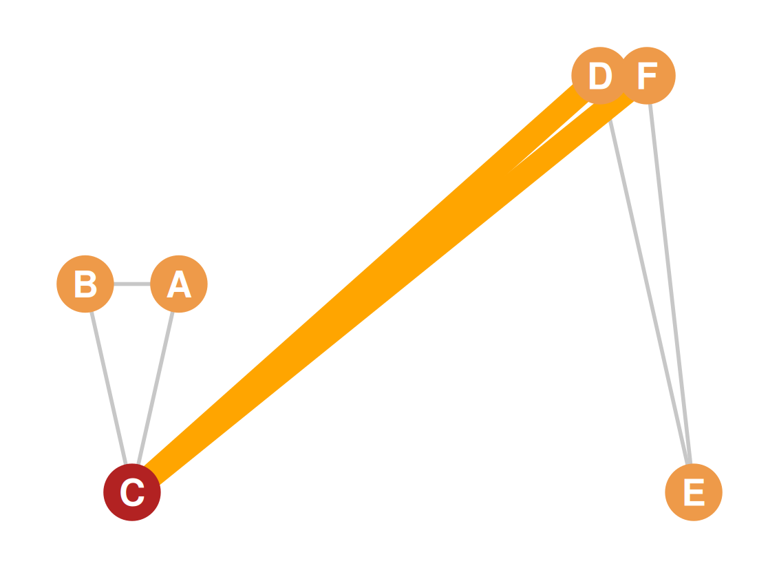
Node cutsets

  • In a graph, any set of nodes that when removed disconnects the graph is called a node cutset
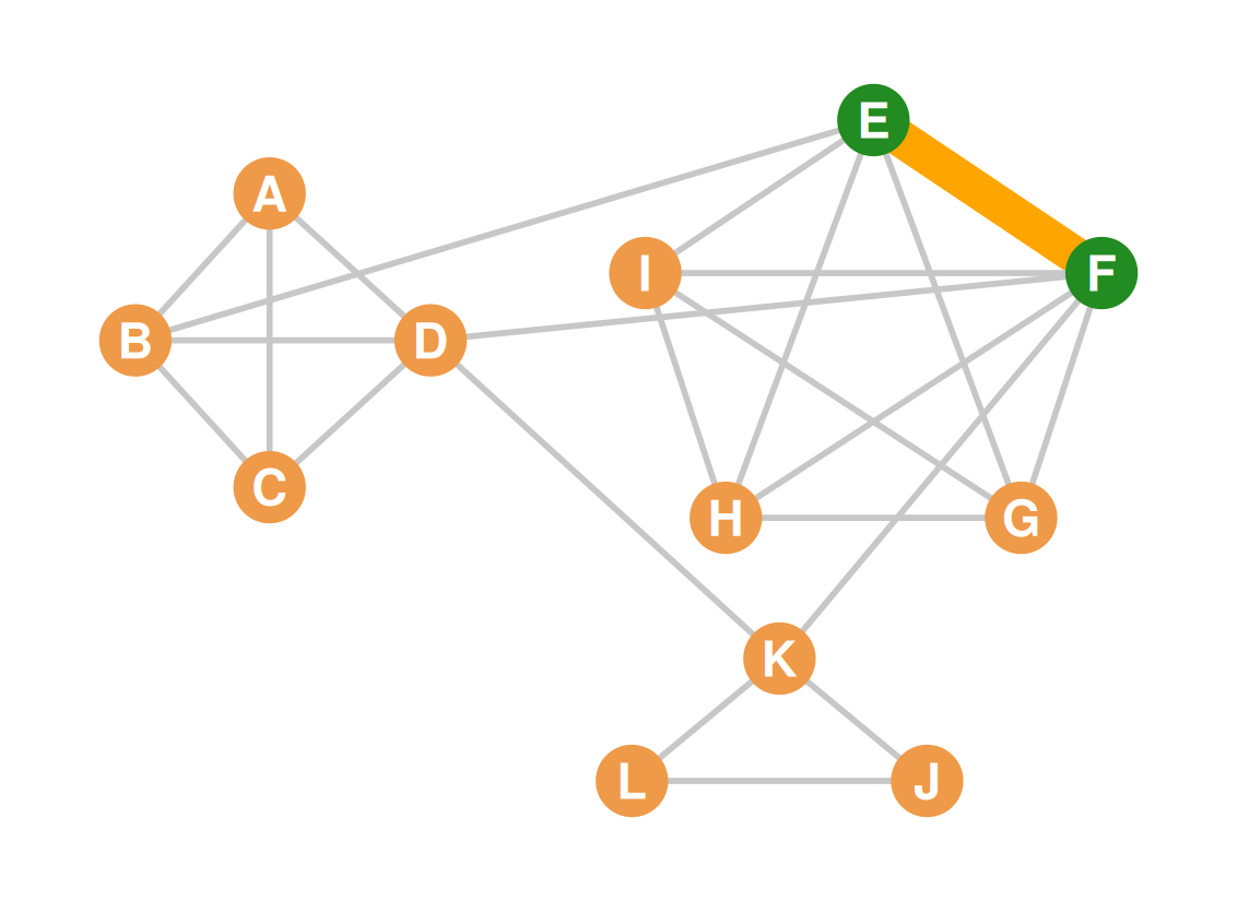
Node cutsets

  • \(\{E, F\}\) is a node cutset for this graph
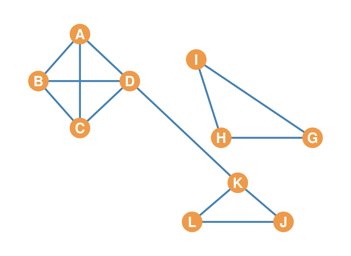
Node cutsets

  • \(\{B, D\}\) is another node cutset for this graph
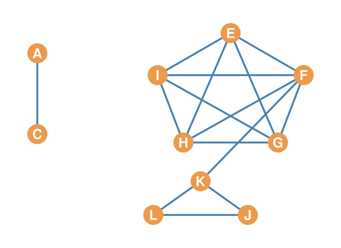
Node cutsets

  • Can you spot another node cutset?

Node cutsets and k-connectivity

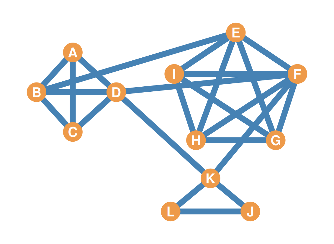
  • The cardinality of the smallest (minimum) node cutset is the same as the graph’s \(k\)-connectivity
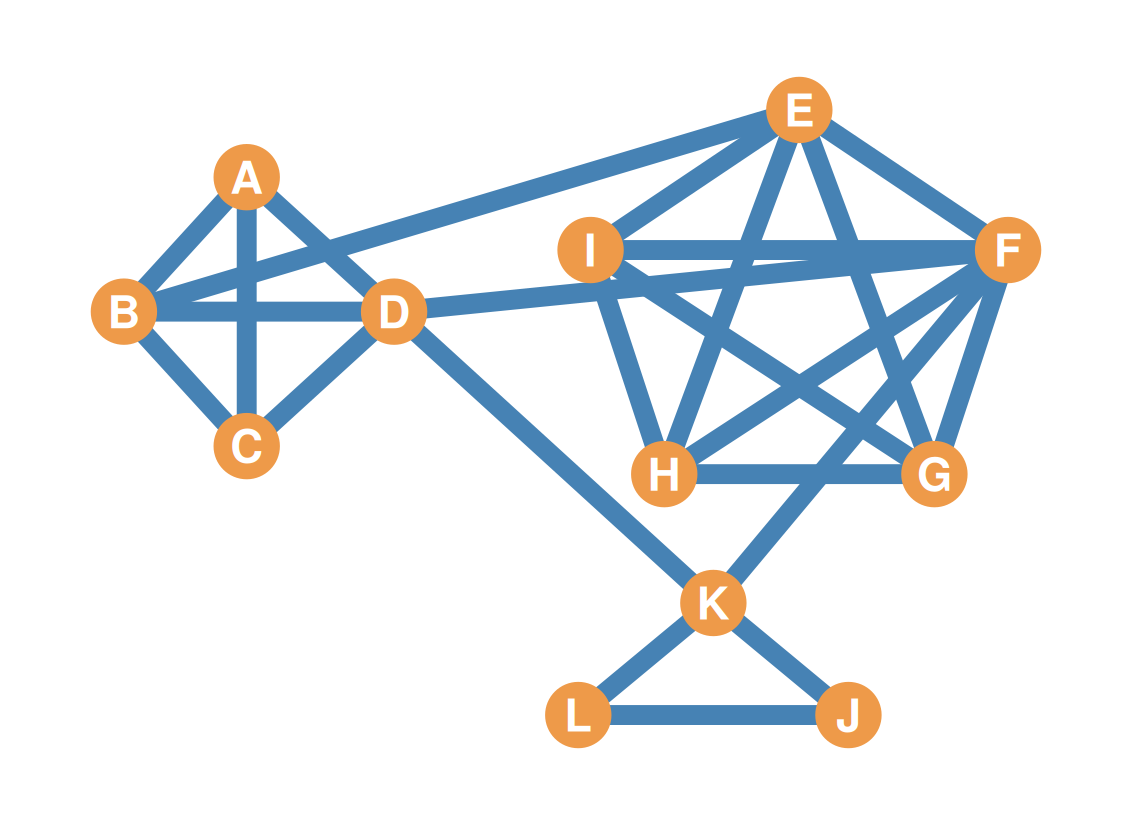
  • What is the \(k\)-connectivity of this graph?
Node cutsets and k-connectivity

  • That’s right! \(k\)-connectivity = 1
  • \(|\{K\}| = 1\): removing the single node \(K\) disconnects the graph
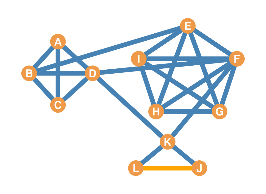
Adding even one edge can raise k-connectivity

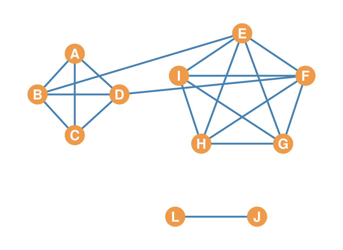
  • Adding even one edge to a graph can increase its \(k\)-connectivity
  • Add the edge \(JL\): now removing \(K\) leaves \(J\) and \(L\) connected, and no single node disconnects the graph
  • \(k\)-connectivity = 2!

Edge cutsets

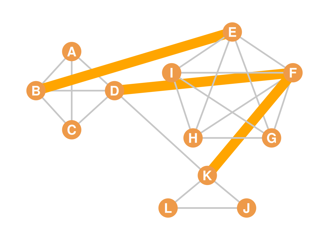
  • In a graph, any set of edges that when removed disconnects the graph is called an edge cutset
  • In this graph \(\{BE, DF, FK\}\) is an edge cutset
Edge cutsets

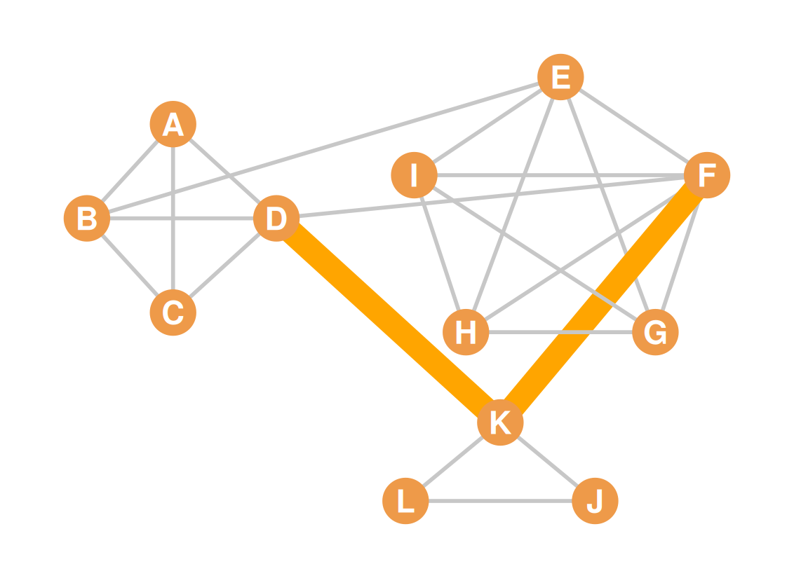
  • \(\{DK, FK\}\) is also an edge cutset

Edge cutsets

  • Can you spot another edge cutset?

Edge cutsets and edge connectivity

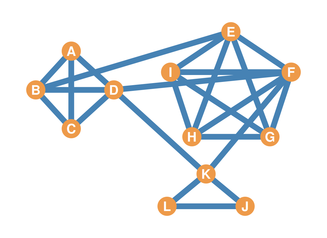
  • The cardinality of the smallest (minimum) edge cutset is the same as the graph’s edge connectivity
  • What is the edge connectivity of this graph?
Edge cutsets and edge connectivity

  • Edge connectivity = 2!
  • \(|\{DK, FK\}| = 2\)
  • \(|\{KJ, KL\}| = 2\)
  • \(|\{JL, KL\}| = 2\)

Menger’s theorem

  • Menger’s theorem states that if a graph has \(k\)-connectivity \(= n\):
    • There are at least \(n\) paths that don’t share nodes connecting every non-adjacent pair of nodes
    • The \(k\)-connector nodes stand on each of these paths
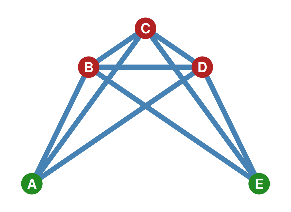
  • This graph has \(k\)-connectivity = 3 (removing the three red nodes disconnects the graph)
Menger’s theorem: counting the paths

  • The two non-adjacent green nodes are indirectly connected in three separate (node-independent) ways!
    • Path 1: \(A \to B \to E\)
    • Path 2: \(A \to C \to E\)
    • Path 3: \(A \to D \to E\)
  • This is an important result in graph theory!
Menger’s theorem: independent paths

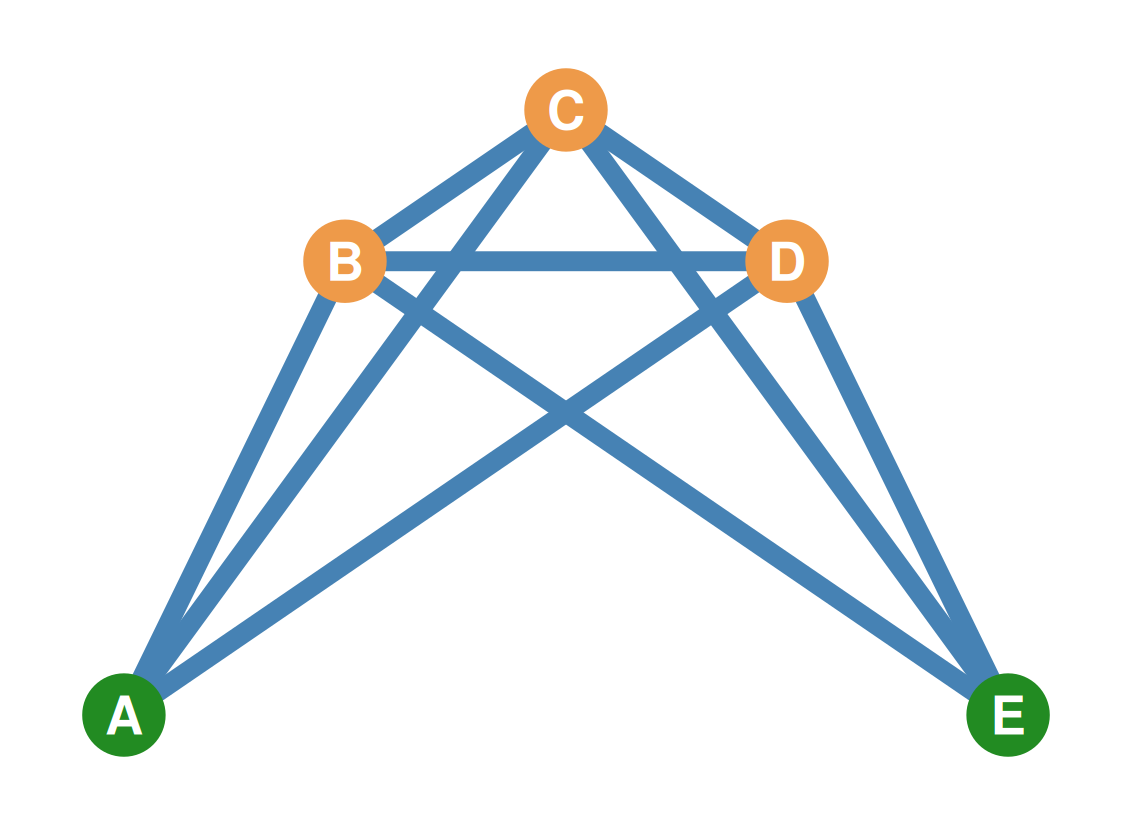
  • In a graph, paths that don’t share nodes are called node-independent paths
  • And paths that don’t share edges are called edge-independent paths
  • Another way of stating Menger’s theorem:
    • If a graph has \(k\)-connectivity \(= n\), there are at least \(n\) node-independent paths connecting each pair of non-adjacent nodes in the graph!

Pairwise node connectivity

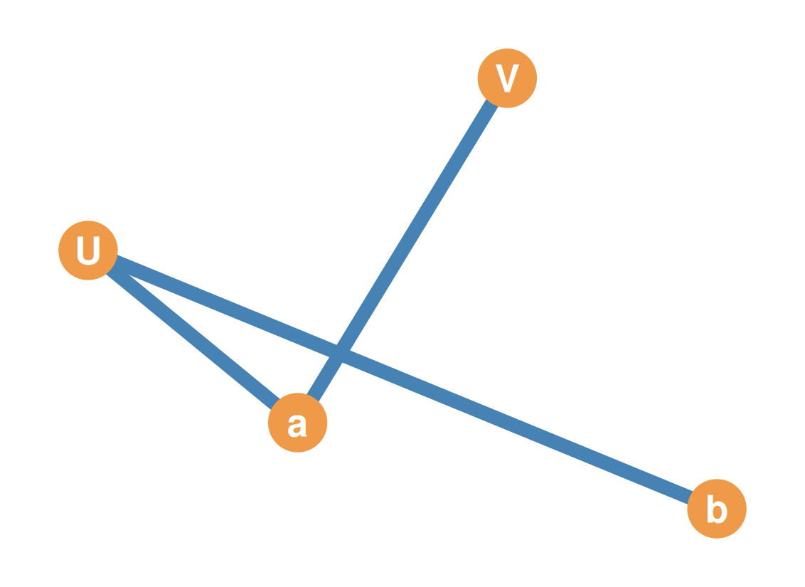
  • For any pair of non-adjacent nodes, \(u\) and \(v\):
  • The pairwise node cutset \(\kappa_{uv}\) is the number of nodes that would have to be removed for them to be disconnected
  • If \(\kappa_{uv} = n\), that means there are at least \(n\) node-independent paths linking \(u\) and \(v\)
  • Two paths are node-independent wherever the inner nodes in each path are different
Pairwise node connectivity

  • \(\kappa_{uv} = 1\): one intermediary node sits on the only path linking \(u\) and \(v\)
  • \(\kappa_{uv} = 2\): two node-independent paths (two separate pairs of inner nodes)
  • \(\kappa_{uv} = 3\): three node-independent paths
Pairwise node connectivity

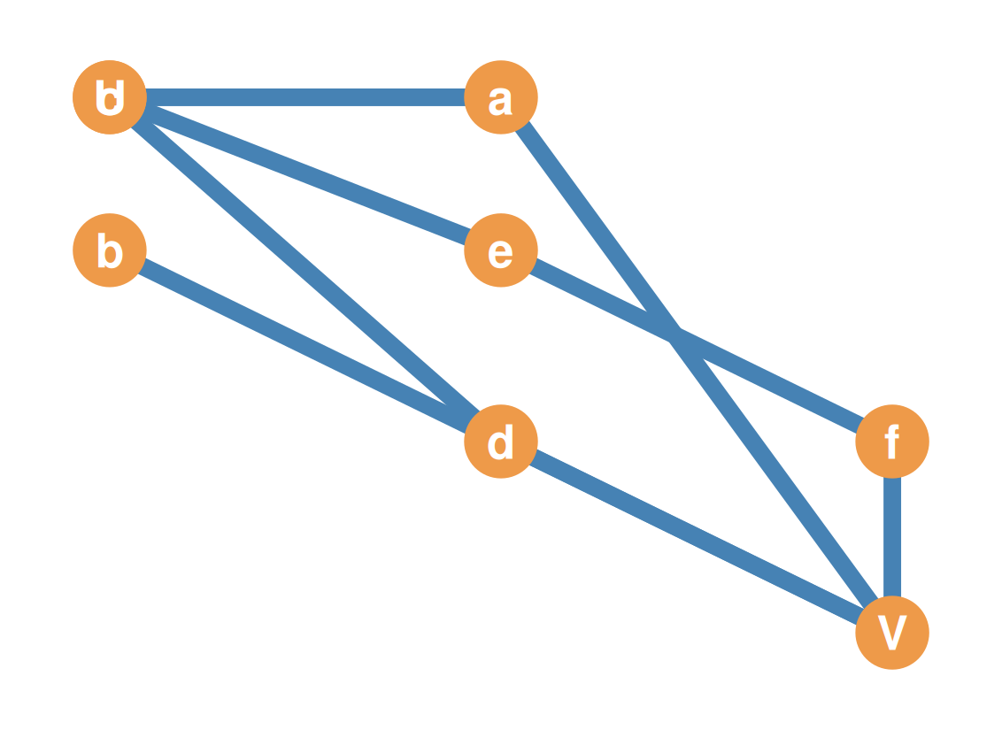
  • \(\kappa_{uv} = 2\): two node-independent paths
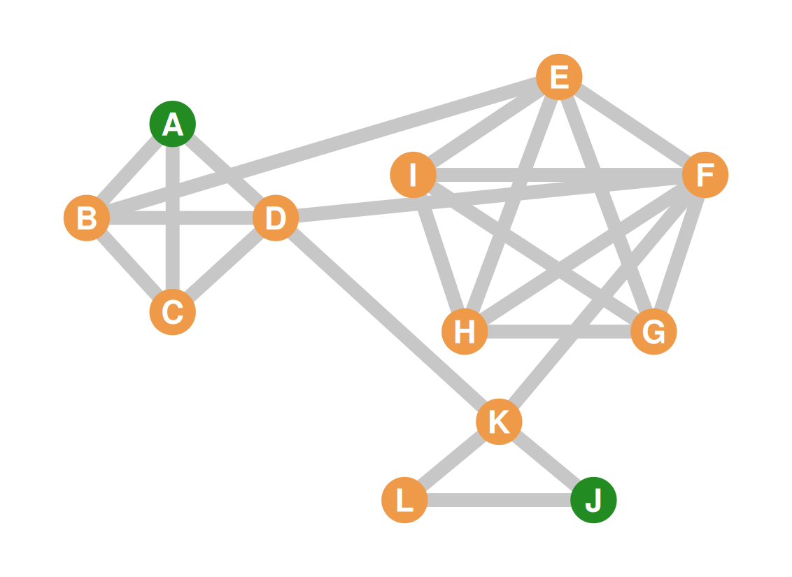
  • In the 12-node graph: \(A\) and \(J\) are non-adjacent, and every path between them passes through \(K\), so \(\kappa_{AJ} = 1\)
Part 6: Cohesion

Graph connectivity as social cohesion

  • \(k\)-connectivity (graph theory) can represent the concept of social cohesion (network theory):
    • The larger the (edge, node) cutset, the more cohesive (integrated) groups are with one another
    • The smaller the (edge, node) cutset, the less cohesive and more potentially fragmented the group structure is

Graph connectivity as social cohesion

  • The more \(k\)-connectivity, the more cohesive (integrated) the group
    • More people would have to be removed to disrupt the group
  • Any graph can be split into subgraphs with any given level of \(k\)-connectivity

Peeling a graph by k-connectivity

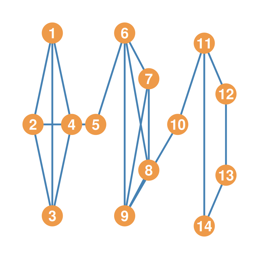
  • \(K = 0\): this graph is already disconnected!
Peeling a graph by k-connectivity

  • \(K = 0\): already disconnected!
  • \(K = 1\): remove the articulation nodes (\(5\) and \(10\)) and the graph falls apart
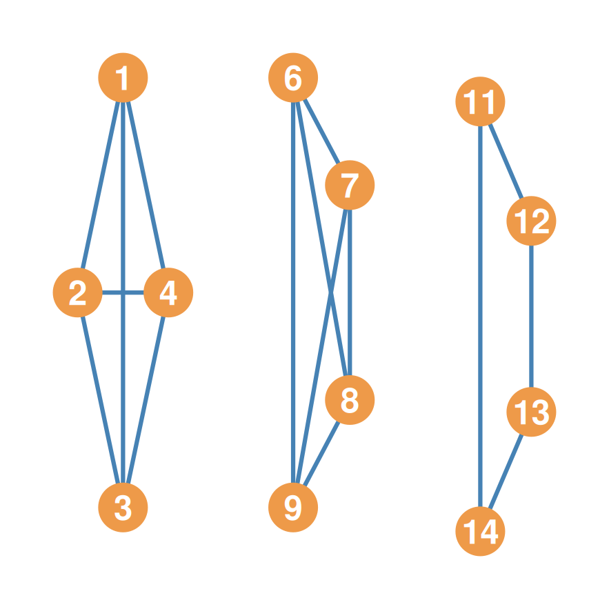
Peeling a graph by k-connectivity

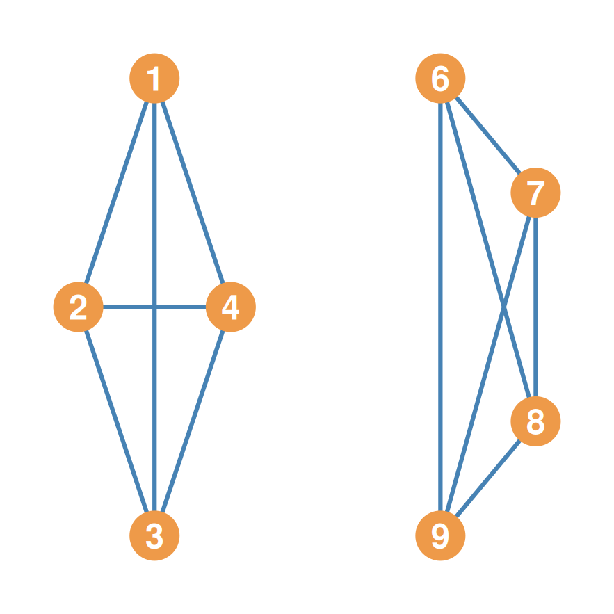
  • \(K = 2\): removing any two nodes of the four-cycle (\(\{11, 12, 13, 14\}\)) disconnects it
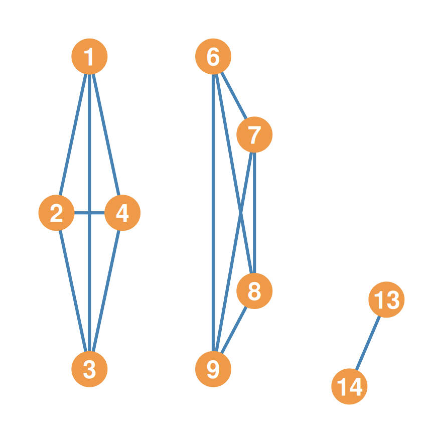
Peeling a graph by k-connectivity

  • \(K = 3\): only the two complete subgraphs remain, the most cohesive structures in the graph
Part 7: Cohesive Blocking

Cohesive blocking

  • The idea of cutsets leads to the Cohesive Blocking approach for the identification of nested cohesive subgroups (Moody and White 2003):
    1. Identify the \(k\)-connectivity of the input graph
    2. Remove the \(k\)-cutset (vertices)
    3. Do the same on the resulting subgraphs until no more subdivisions can be obtained

Cohesive blocking: the input graph

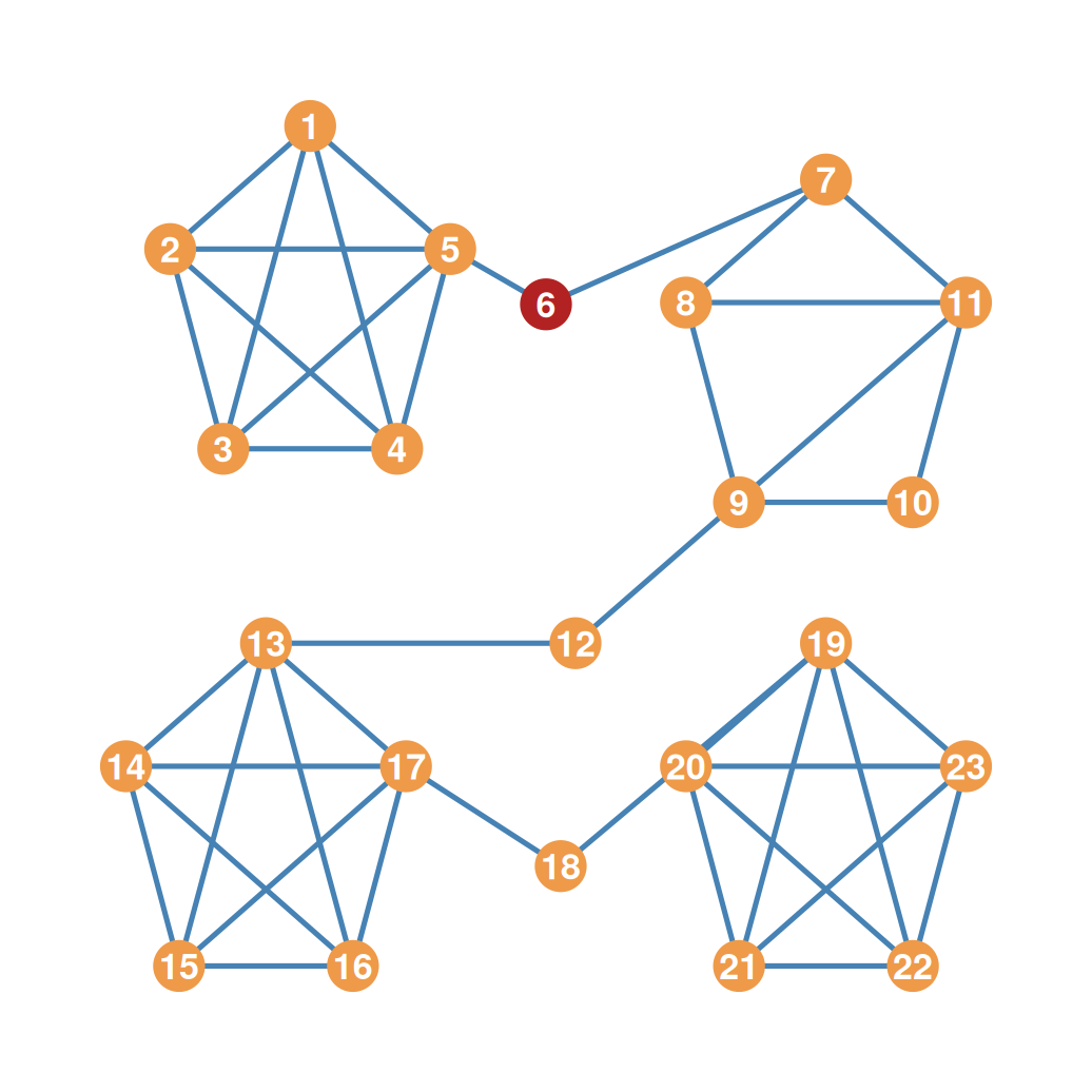
  • This 23-node graph \(G\) is 1-node connected!
  • Can you tell which node we need to remove?
Cohesive blocking: remove the cutset

  • Removing node 6 splits \(G\) into two subgroups:
    • \(\{1, 2, 3, 4, 5\}\)
    • \(\{7, 8, ..., 23\}\)
  • Now identify the \(k\)-connectivity of each
Cohesive blocking: recursion

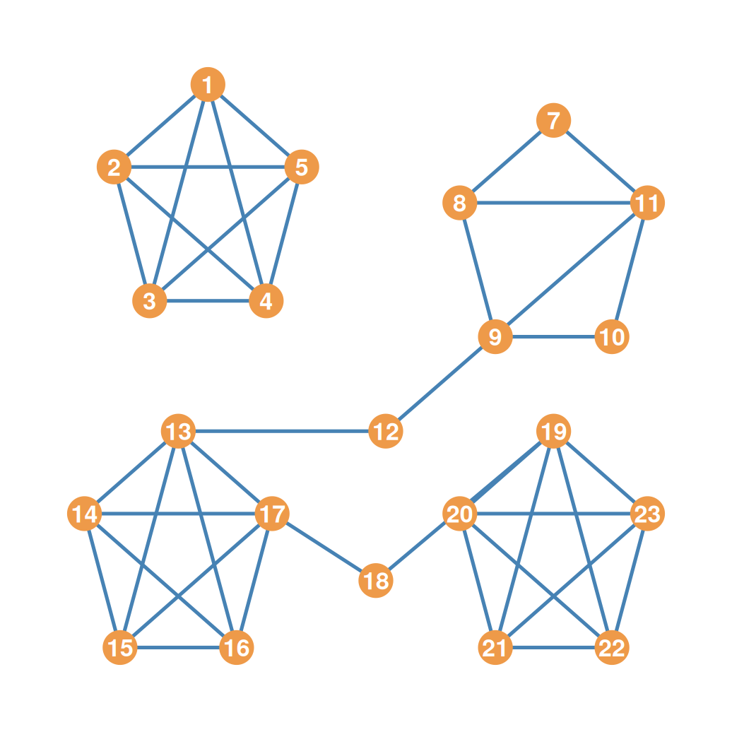
  • The subgroup \(\{7, ..., 23\}\) is 1-connected: remove node 12
  • The subgroup \(\{1, ..., 5\}\) is a clique (\(k\)-connectivity = 4): stop
Cohesive blocking: recursion (cont.)

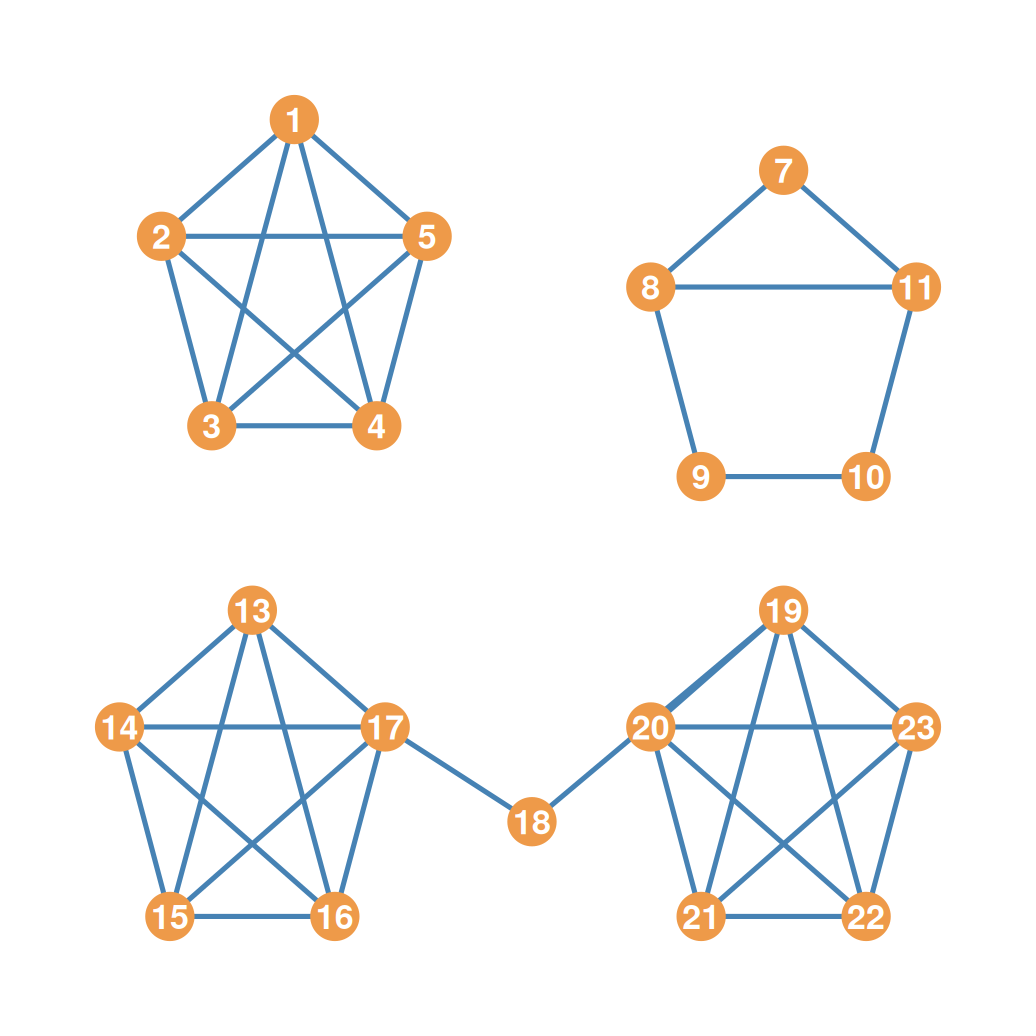
  • The subgroup \(\{13, ..., 23\}\) is 1-connected: remove node 18
  • The subgroup \(\{7, ..., 11\}\) is a cycle (\(k\)-connectivity = 2): stop
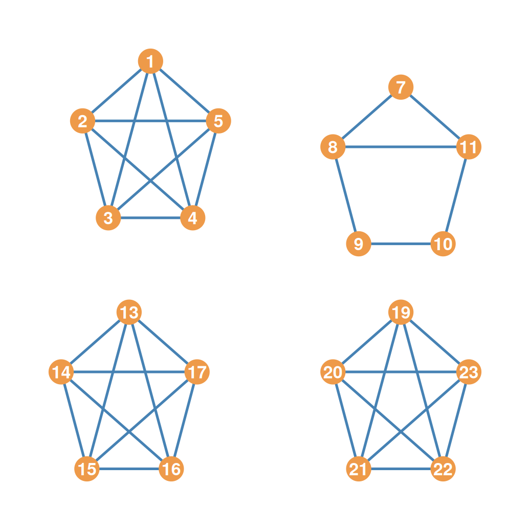
The cohesive blocking tree

  • The algorithm yields a tree of nested cohesive subgroups:
    • \(G\) (\(k = 1\))
      • \(\{1, ..., 5\}\) (\(k = 4\), a clique)
      • \(\{7, ..., 23\}\) (\(k = 1\))
        • \(\{7, ..., 11\}\) (\(k = 2\), a cycle)
        • \(\{13, ..., 23\}\) (\(k = 1\))
          • \(\{13, ..., 17\}\) (\(k = 4\), a clique)
          • \(\{19, ..., 23\}\) (\(k = 4\), a clique)
  • Deeper blocks are more cohesive: more members would have to be removed to break them
Members K
G {1,2,3,4,5,6,7,8,9,10,11,12,13,14,15,16,17,18,19,20,21,22,23} 1
B1 {1,2,3,4,5} 4
B2 {7,8,9,10,11,12,13,14,15,16,17,18,19,20,21,22,23} 1
B3 {7,8,9,10,11} 2
B4 {13,14,15,16,17,18,19,20,21,22,23} 1
B5 {13,14,15,16,17} 4
B6 {19,20,21,22,23} 4

Part 8: Lambda Sets

Using edge connectivity to find cohesive subsets

  • We can use pairwise edge connectivity \(\lambda(u, v)\) to recursively find Lambda Sets (Borgatti, Everett, & Shirey, 1990).
  • The core property of lambda sets:
    • The pairwise edge connectivity between nodes inside a lambda set is always strictly larger than the edge connectivity between any node inside the set and any node outside the set.
    • This mathematically guarantees that group members have stronger indirect ties with each other than with any outsider!
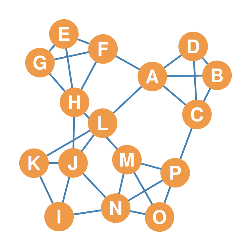
  • Let’s walk through the hierarchical partition algorithm on a 16-node graph.

Lambda sets: step-by-step splitting

  • Step 1: start with graph \(G\). Its edge connectivity is \(\lambda(G) = 3\); removing the minimum edge cutset \(\{AF, AL, CP\}\) splits the graph.
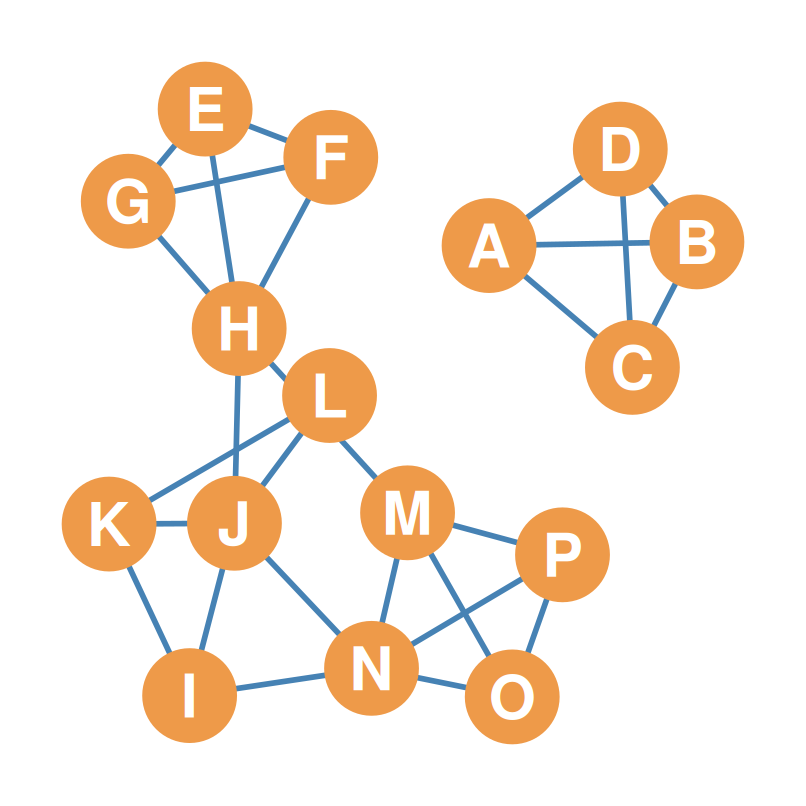
Lambda sets: step-by-step splitting

  • Step 2: remove \(\{AF, AL, CP\}\). This splits the graph into a clique component \(\{A, B, C, D\}\) (\(\lambda = 3\)) and a giant component (\(\lambda = 2\)).
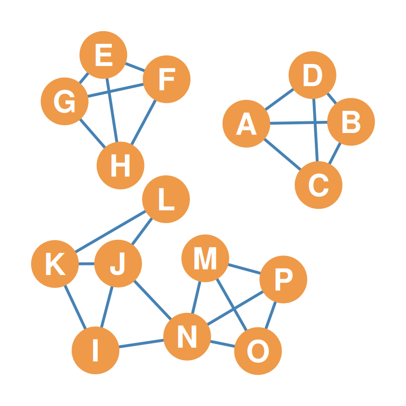
Lambda sets: step-by-step splitting (cont.)

  • Step 3: remove \(\{HJ, HM\}\). This disconnects the giant component, yielding a new component and a clique of size 4.
Lambda sets: step-by-step splitting (cont.)

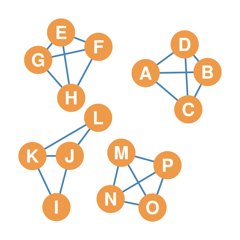
  • Step 4: remove \(\{JN, IN\}\). Disconnecting the final remaining components reveals four cohesive subgroups (cliques of size 4).
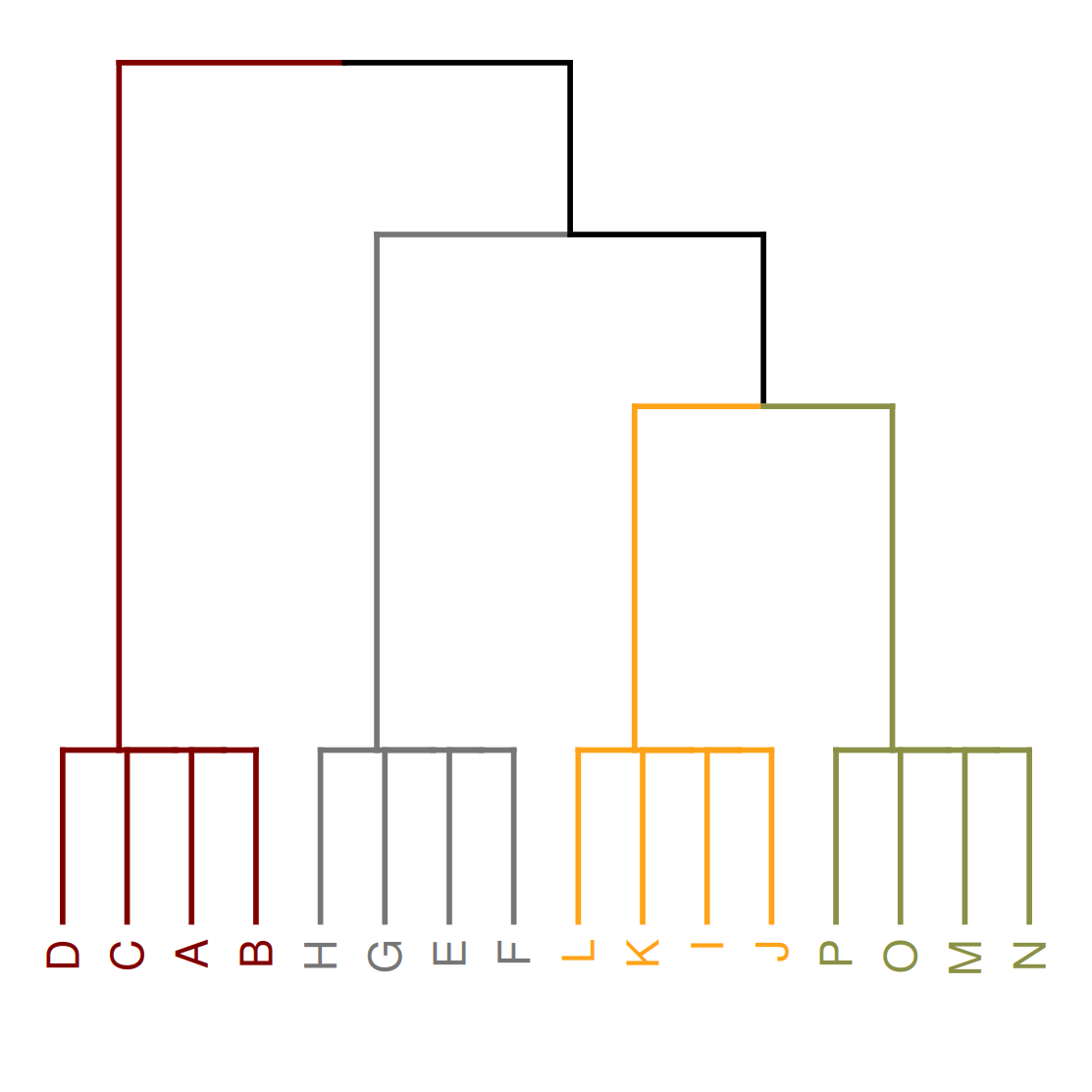
Dendrogram of lambda sets

  • Because lambda sets are hierarchically nested, we can plot their nested relationship using a dendrogram.
  • Properties of lambda sets:
    • At any given partition height, each node belongs to exactly one lambda set.
    • Smaller, tighter lambda sets are cleanly nested within larger, looser ones.
    • Excellent for showing multi-level nested structures (e.g., departments nested in divisions, nested in the firm).
Part 9: K-Core Decomposition & Core-Periphery Structures

Core-periphery structures

  • Sometimes networks are organized so that there is a cohesive subgroup hidden inside a set of less well-connected nodes
  • The cohesive subgroup is called the core
  • The other nodes are called the periphery
  • These are called core-periphery structures
K-core decomposition: the onion method

  • The method of \(k\)-core decomposition helps us find well-connected cores in networks:
    1. Begin with the less well-connected nodes (e.g., degree = 1)
    2. Remove those
    3. Continue removing nodes based on degree to reveal deeper “shells” (like an onion)
    4. Find the hidden core!

K-core decomposition: k = 0

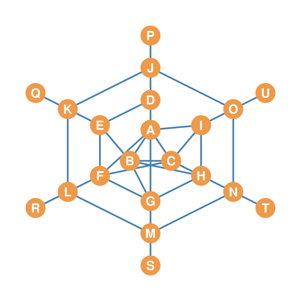
  • Start with the full 21-node network

K-core decomposition: k = 1

  • Remove the least well-connected nodes first: the six pendant nodes (\(P\) to \(U\))
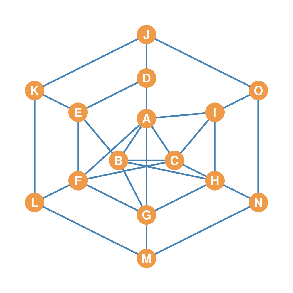
K-core decomposition: k = 2

  • Continue peeling: the six cycle nodes (\(J\) to \(O\)) now have the lowest degree
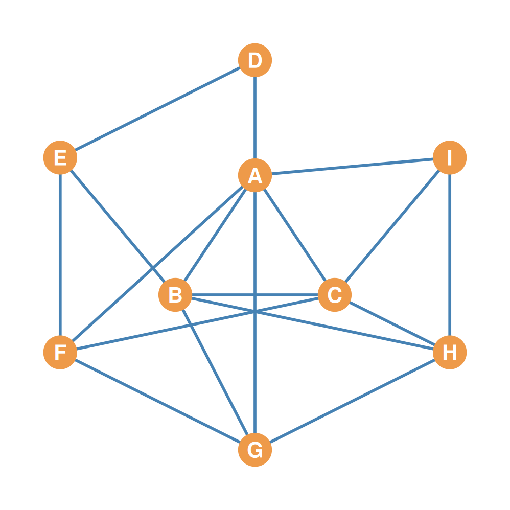
K-core decomposition: k = 3

  • The next shell (\(B\), \(D\), \(F\), \(G\), \(H\), \(I\)) comes off
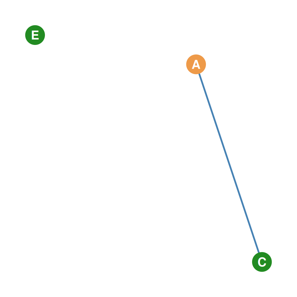
K-core decomposition: the core

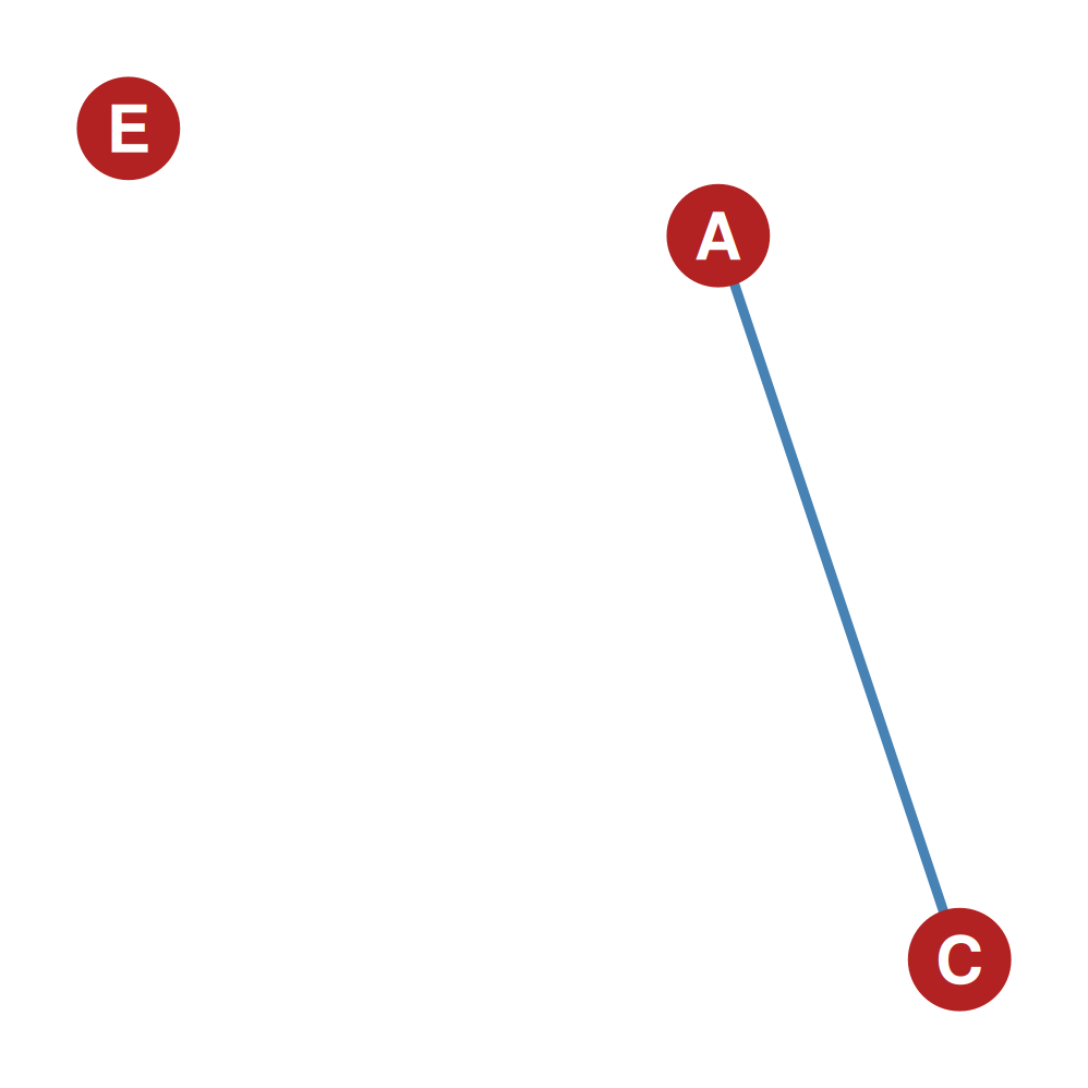
  • Nodes \(A\), \(C\), and \(E\) are the core of this network
  • Everything else was periphery, peeled away shell by shell
Mathematical core-periphery models

  • To formally test for core-periphery structures, we fit ideal blockmodels to our observed adjacency matrix:
  • Ideal core-periphery adjacency matrix:
    • The Core block is a 1-block (density \(\approx\) 1.0).
    • The Core-to-Periphery blocks are 1-blocks (density \(\approx\) 1.0, periphery is tied to the core).
    • The Periphery-to-Periphery block is a 0-block (density \(\approx\) 0.0, peripheral nodes do not connect).
  • \[ \mathbf{Adj} = \begin{pmatrix} \mathbf{Core} & \mathbf{Core/Periph} \\ \mathbf{Periph/Core} & \mathbf{Periphery} \end{pmatrix} = \begin{pmatrix} \mathbf{1} & \mathbf{1} \\ \mathbf{1} & \mathbf{0} \end{pmatrix} \]
  • This mathematical structure allows us to predict network outcomes and analyze systemic robustness.

Part 10: Summary of Key Terms

Summary of key terms (I)

  • Subgraph: A subset (\(G'\)) of the node and the edge set of a graph (\(G\))
  • Connected subgraph: All nodes in the subgraph can reach other nodes in the subgraph via some path within the subset of edges
  • Maximal subgraph: A subgraph is maximal with respect to property \(p\) (e.g., completeness, connectivity) when no more nodes or edges can be added to the subgraph without losing that property
    • Maximally connected subgraph, maximally complete subgraph, etc.
  • Clique: Maximally complete subgraph
  • Clique size: Number of nodes in a clique
  • \(n\)-Clique: A subgraph in which every node can reach every other node inside the subgraph via a path of minimum length \(n\)

Summary of key terms (II)

  • Connected graph: All nodes in the graph can reach every other node via a path regardless of length (\(l < \infty\))
  • Disconnected graph: Some nodes in the graph cannot reach other nodes via any path (e.g., for at least one pair of nodes \(l_{uv} = \infty\))
  • Components: Maximally connected subgraphs inside a disconnected graph
  • Giant component: The maximally connected subgraph in a disconnected graph with the largest number of nodes
  • \(k\)-Connected component: A component in which every node can reach every other node inside the component via a path of minimum length \(k\)

Summary of key terms (III)

  • Bridges: An edge that if it were removed would disconnect the graph
  • Edge cutset: Minimum number of edges whose removal would disconnect the graph
  • Node cutset: Minimum number of nodes whose removal would disconnect the graph
  • uv-cutset: Number of nodes whose removal would disconnect a pair of nodes (\(uv\))
  • Menger’s theorem: If a graph has \(k\)-connectivity \(= n\), every pair of non-adjacent nodes is connected by at least \(n\) node-independent paths
  • Cohesive blocking: A way to find densely connected subgroups in a graph by removing nodes in the node cutset (Moody & White 2003)