Small-World Transitions

This page details a computational experiment on how distinction centrality evolves as a network transitions from a perfectly symmetric, highly constrained structure to a fully saturated, completely connected structure.

Simulation Setup

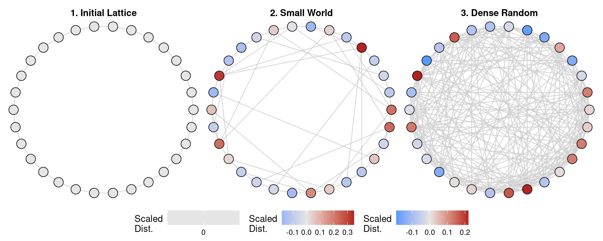
We begin with a regular lattice (a circle graph or ring) of size \(N = 30\). Because the graph is node-transitive, every node is structurally equivalent. Under the absolute maximum (abm) normalization, all nodes experience identical constraint, meaning the variance in distinction is exactly zero.

From this initial state, we progressively add non-existent edges at random until the graph becomes a complete graph (\(K_{30}\)). At each step of the simulation, we recalculate the distinction metrics for the network.

library(igraph)
library(dplyr)
library(ggplot2)
library(ggraph)
library(patchwork)
source("../Functions/distinction.R")

set.seed(42)
N <- 30
g <- make_ring(N)

max_edges <- N * (N - 1) / 2
current_edges <- ecount(g)
edges_to_add <- max_edges - current_edges
steps <- 50
edges_per_step <- floor(edges_to_add / steps)

# Generate a randomized list of all non-existent edges
full_g <- make_full_graph(N)
missing_edges <- difference(full_g, g)
missing_edge_list <- as_edgelist(missing_edges)
missing_edge_list <- missing_edge_list[sample(nrow(missing_edge_list)), ]

# Track metrics
results <- list()
res <- distinction(g, norm = "abm")
results[[1]] <- data.frame(
  step = 0, edges = ecount(g), density = edge_density(g),
  mean_u = mean(res$u), sd_scd = sd(res$scd)
)

# Run simulation
edge_idx <- 1
for (i in 1:steps) {
  n_add <- min(edges_per_step, nrow(missing_edge_list) - edge_idx + 1)
  if (n_add <= 0) break
  edges_to_add_now <- missing_edge_list[edge_idx:(edge_idx + n_add - 1), ]
  edge_idx <- edge_idx + n_add
  
  g <- add_edges(g, as.vector(t(edges_to_add_now)))
  res <- distinction(g, norm = "abm")
  
  results[[i + 1]] <- data.frame(
    step = i, edges = ecount(g), density = edge_density(g),
    mean_u = mean(res$u), sd_scd = sd(res$scd)
  )
}

df_sim <- bind_rows(results)

Structural Snapshots

As we add random long-ties, the network transitions through a “small-world” phase before becoming a dense random graph. The visualization below maps the node color to distinction centrality: from blue (highly constrained/negative distinction) to red (highly distinctive broker).

# Helper function to plot a snapshot
plot_network_snap <- function(g, title) {
  V(g)$name <- as.character(1:vcount(g))
  res <- distinction(g, norm = "abm")
  
  layout_coords <- layout_in_circle(g)
  
  ggraph(g, layout = layout_coords) +
    geom_edge_link(color = "gray80", width = 0.5, alpha = 0.7) +
    geom_node_point(aes(fill = res$scd), shape = 21, size = 5, color = "black") +
    scale_fill_gradient2(low = "dodgerblue", mid = "gray90", high = "firebrick", name = "Scaled\nDist.") +
    labs(title = title) +
    theme_void() +
    theme(plot.title = element_text(hjust = 0.5, size = 11, face = "bold"),
          legend.position = "bottom")
}

# Recreate specific phases for visualization
g1 <- make_ring(N)
g2 <- add_edges(g1, as.vector(t(missing_edge_list[1:25, ])))
g3 <- add_edges(g1, as.vector(t(missing_edge_list[1:200, ])))

p1 <- plot_network_snap(g1, "1. Initial Lattice")
p2 <- plot_network_snap(g2, "2. Small World")
p3 <- plot_network_snap(g3, "3. Dense Random")

p1 + p2 + p3 + plot_layout(ncol = 3, guides = "collect") & theme(legend.position = 'bottom')

Evolution of Distinction Variance (Inequality)

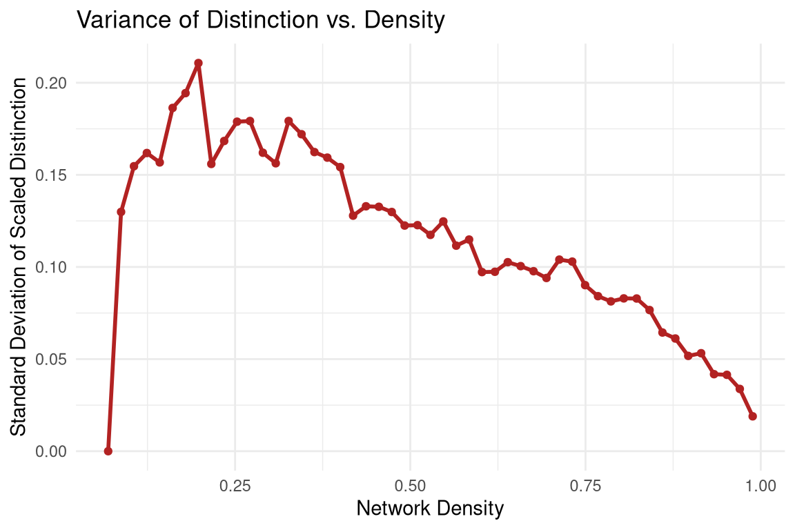
Structural inequality in distinction follows a clear inverted U-shape. At zero density (the regular lattice) and full density (the complete graph), the variance is exactly zero. However, in the sparse, clumpy “small-world” regime, a few nodes become highly distinctive brokers while others remain locally constrained, causing structural inequality to hit its absolute peak.

ggplot(df_sim, aes(x = density, y = sd_scd)) +
  geom_line(color = "firebrick", linewidth = 1) +
  geom_point(color = "firebrick", size = 1.5) +
  labs(x = "Network Density", y = "Standard Deviation of Scaled Distinction",
       title = "Variance of Distinction vs. Density") +
  theme_minimal()

Evolution of Baseline Constraint

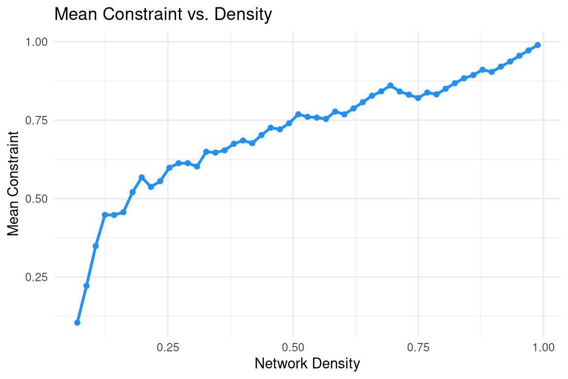
Mean constraint follows a monotonically increasing curve. As edges are added, nodes are increasingly connected to alters with heterogeneous and higher status scores, thereby increasing the overall structural dependence on neighbors. This constraint eventually asymptotes to exactly \(1.0\) in the complete graph.

ggplot(df_sim, aes(x = density, y = mean_u)) +
  geom_line(color = "dodgerblue", linewidth = 1) +
  geom_point(color = "dodgerblue", size = 1.5) +
  labs(x = "Network Density", y = "Mean Constraint",
       title = "Mean Constraint vs. Density") +
  theme_minimal()