Exploratory Analysis Showcase

This page provides a quick showcase of exploratory analysis using the cleaned SSI-2012 dataset. We illustrate basic data distributions and aesthetic tastes using clean, standard visualizations in R.

1. Classical Music Tastes

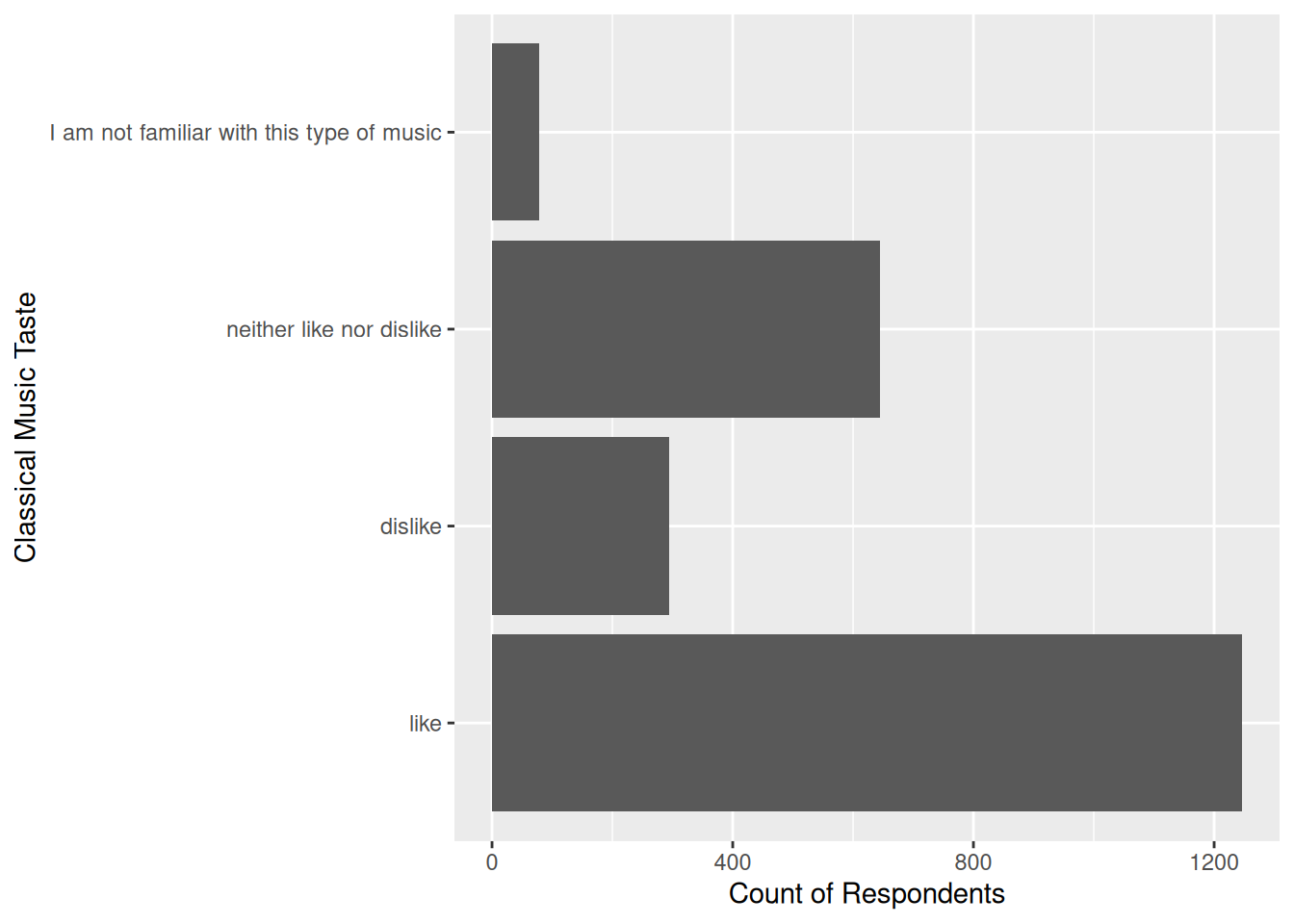
Let’s examine how respondents rate their liking of Classical music (classicaltaste). This variable has four main levels: like, dislike, neither like nor dislike, and I am not familiar with this type of music.

# Convert classicaltaste to standard factor for plotting
df_classical <- df |> 
  filter(!is.na(classicaltaste)) |> 
  mutate(classicaltaste = as_factor(classicaltaste))

# Create bar chart with aesthetic mapping to y-axis (avoiding coord_flip)
ggplot(df_classical, aes(y = classicaltaste)) +
  geom_bar() +
  labs(
    x = "Count of Respondents",
    y = "Classical Music Taste"
  )

Figure 1: Distribution of Classical Music Tastes among respondents.

As shown in Figure 1, a substantial majority of the 2,276 respondents report that they like Classical music, while only a small percentage are completely unfamiliar with it.

---

2. Subjective Social Class Self-Identification

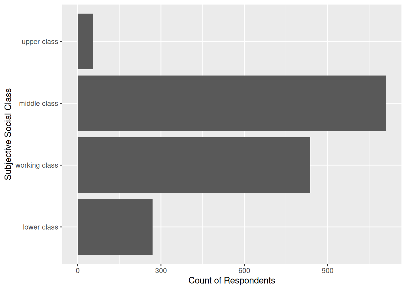
Respondents were asked: “Which of these do you think best describes you?” with options: lower class, working class, middle class, and upper class (percclass).

# Convert percclass to factor and filter missing values
df_class <- df |> 
  filter(!is.na(percclass)) |> 
  mutate(percclass = as_factor(percclass))

# Plot distribution
ggplot(df_class, aes(y = percclass)) +
  geom_bar() +
  labs(
    x = "Count of Respondents",
    y = "Subjective Social Class"
  )

Figure 2: Self-described subjective social class of respondents.

As displayed in Figure 2, the majority of respondents identify as middle class or working class, with smaller proportions self-identifying as lower class or upper class.

---

3. Painting Impression Ratings (Pre-Test)

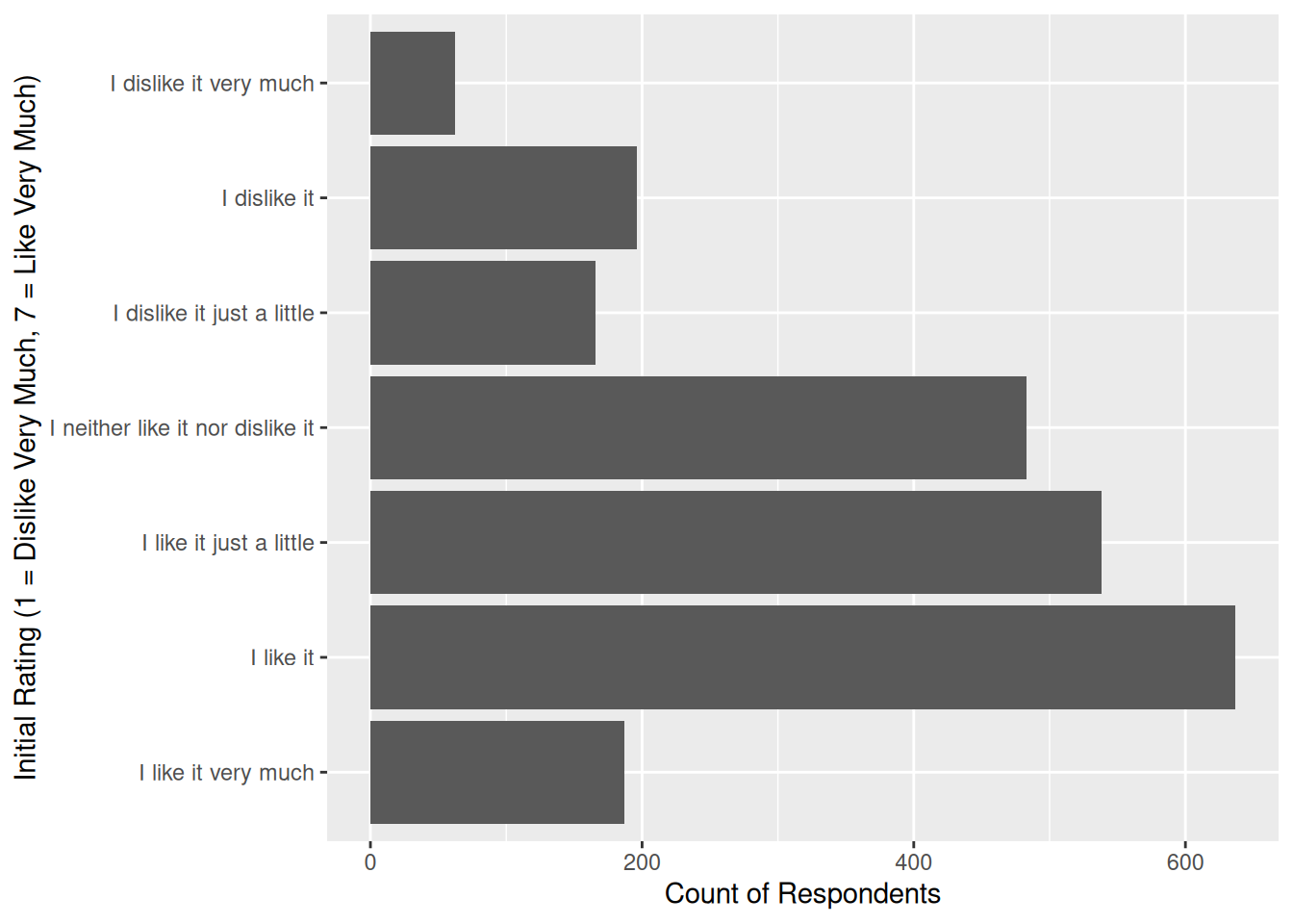
Before receiving any social manipulation, respondents gave their first impression of an abstract painting on a scale from 1 (dislike very much) to 7 (like very much) (taste1).

# Convert taste1 to standard factor to represent its ordinal categories
df_painting <- df |> 
  filter(!is.na(taste1)) |> 
  mutate(taste1_factor = as_factor(taste1))

ggplot(df_painting, aes(y = taste1_factor)) +
  geom_bar() +
  labs(
    x = "Count of Respondents",
    y = "Initial Rating (1 = Dislike Very Much, 7 = Like Very Much)"
  )

Figure 3: Distribution of initial painting taste ratings (1-7 scale).

The pre-test ratings shown in Figure 3 reveal a wide distribution of opinions on the painting, peaking in the neutral and mild liking ranges.