1 Social Network Surveys

This section describes the dyadic social network surveys and weekly aggregated network metrics. You can download the complete datasets and survey instruments below:

Download CSV Dataset (.csv) Download R Dataset (.rds) Download Stata Dataset (.dta)

Interactive Survey Instruments & Original Questionnaires

Explore the digitized interactive codebooks and original LimeSurvey PDF instruments for each wave below:

• Wave 1: Summer 2011 Network Survey ( PDF)

• Wave 2: Spring 2012 Network Survey ( PDF)

• Wave 3: Summer 2012 Network Survey ( PDF)

• Wave 4: Fall 2012 Network Survey ( PDF)

• Wave 5: Winter 2013 Network Survey ( PDF)

• Wave 6: Summer 2013 Network Survey ( PDF)

• Weekly Aggregated Metrics: Located in Data/weekly_aggregated_metrics/ (Contains open .csv files tracking participant indegrees, outdegrees, and text/voice communication inflow and outflow across academic weeks).

The network survey asked students to nominate their peers and answer detailed questions about their relationship with each peer. These nominations represent directed ties between a nominating ego (sender) and a nominated alter (receiver).

---

1.1 Programmatic Consolidation

Originally, the network surveys were scattered across 9 separate Stata .dta files (representing Wave 1 through Wave 8, including supplementary entry Wave 7.2).

A custom R consolidation script (Code/consolidate_network_surveys.R) was engineered to: 1. Parse the wave identifiers from the file names. 2. Programmatically drop sensitive identifying information (such as altername and receiver_string). 3. Strip wave-specific variable suffixes (e.g., closeness_1, closeness_75, closeness_8 are all renamed to closeness). 4. Harmonize variable types across waves to handle type conflicts safely. 5. Combine all observations into a single longitudinal panel dataset.

---

1.2 Nominations by Wave

Below is an interactive count of dyadic ties (nominations) captured in each wave of the longitudinal panel.

library(readr)
library(dplyr)

# Load consolidated network surveys
net_df <- read_csv("Data/network_surveys_longitudinal_clean.csv", show_col_types = FALSE)

# Generate count table
net_df |>
  group_by(Wave = wave) |>
  summarise(
    Nominations = n(),
    Unique_Senders = n_distinct(sender),
    Unique_Receivers = n_distinct(receiver)
  ) |>
  arrange(Wave) |>
  knitr::kable(caption = "Tie and Participant Counts by Survey Wave")

Table 1: Tie and Participant Counts by Survey Wave

Wave	Nominations	Unique_Senders	Unique_Receivers
1	264	17	209
2	2490	173	1967
3	2241	175	1735
4	1524	134	1172
5	1514	140	1248
6	1327	124	1067
7	1207	95	998
8	1251	106	1028

---

1.3 Core Relational Attributes

For each nominated tie, participants provided detailed ratings across several dimensions:

• Closeness (closeness): Subjective emotional closeness to the nominee (e.g., on a 1–7 Likert scale).
• Tie Duration (duration): How long they have known each other in years.
• Contact Frequency (freqlast3months, freqlastyear): Frequency of face-to-face and digital communication.
• Emotional Profiles: Specific emotional dimensions of the friendship, such as:
  • emotionloving: Feeling loving/affectionate.
  • emotionexciting: Feeling excited/happy.
  • emotionsignificant: Feeling validated/significant.
• Interaction Contexts (socialcontext*): Where they typically interact (e.g. socialcontextDorm, socialcontextInclass, socialcontextClubteam, socialcontextInternet).
• Shared Activities (activitiesact*, sameactivities*): Activities they do together, such as studying, playing sports, partying, or talking about personal problems.

---

1.4 Descriptive Relational Visualizations

To help visualize how these social ties and emotional dimensions vary across different relationship categories, the consolidated panel was used to generate several standardized profile figures.

1.4.1 Emotional Closeness by Relationship Type

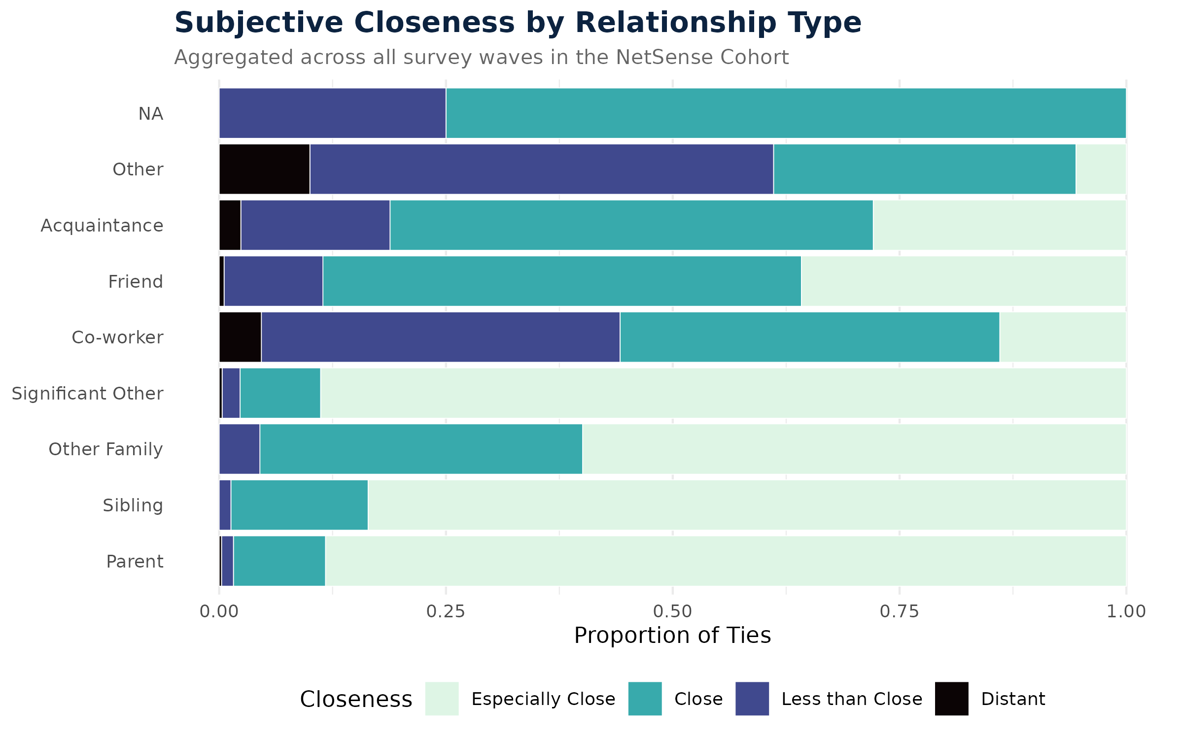
The figure below illustrates the proportion of emotional closeness levels reported within each relationship category. For instance, parents and significant others dominate the “Especially Close” tier, while acquaintances and coworkers represent more “Distant” or “Less than Close” ties.

Figure 1: Subjective Closeness Profiles by Relationship Type

1.4.2 Relationship Duration

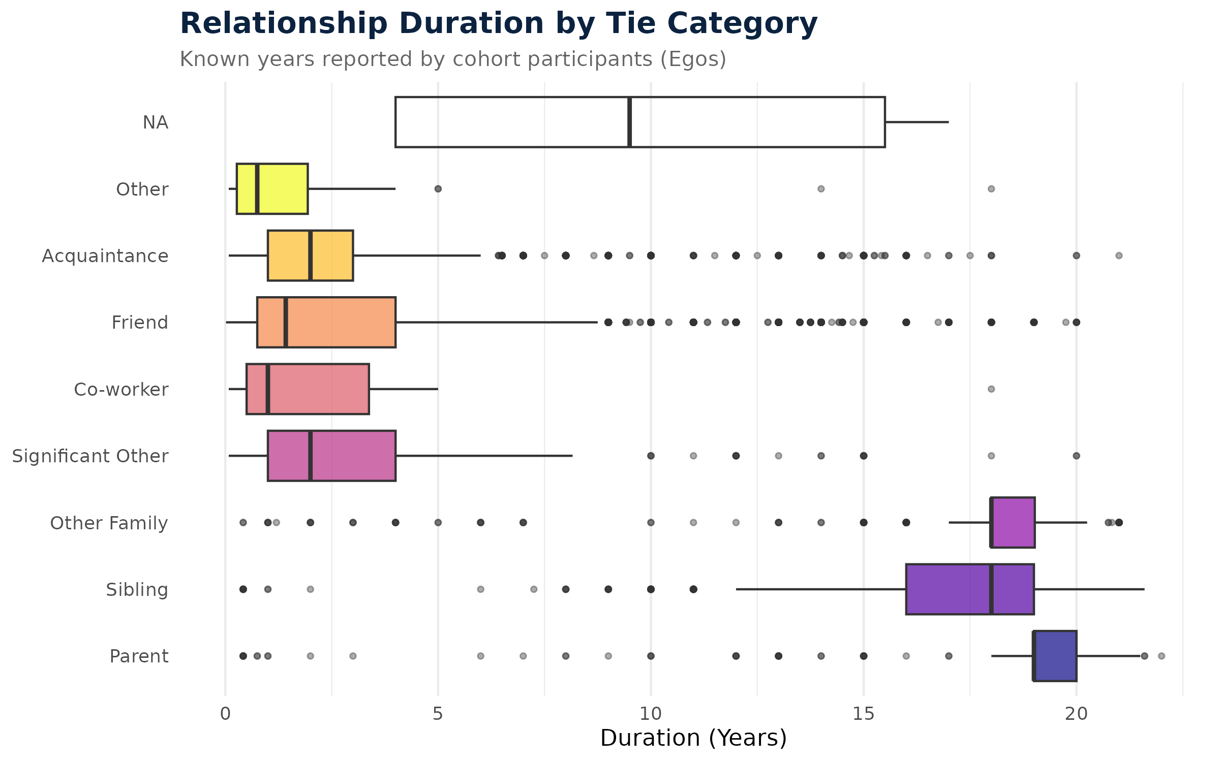
The boxplot below shows the distribution of relationship duration in years across different categories. Naturally, family relationships (parents and siblings) exhibit the longest durations, while friendships and classmate acquaintances reflect shorter, college-coincident spans.

Figure 2: Relationship Durations Across Categories

1.4.3 Emotional Profiles of Social Ties

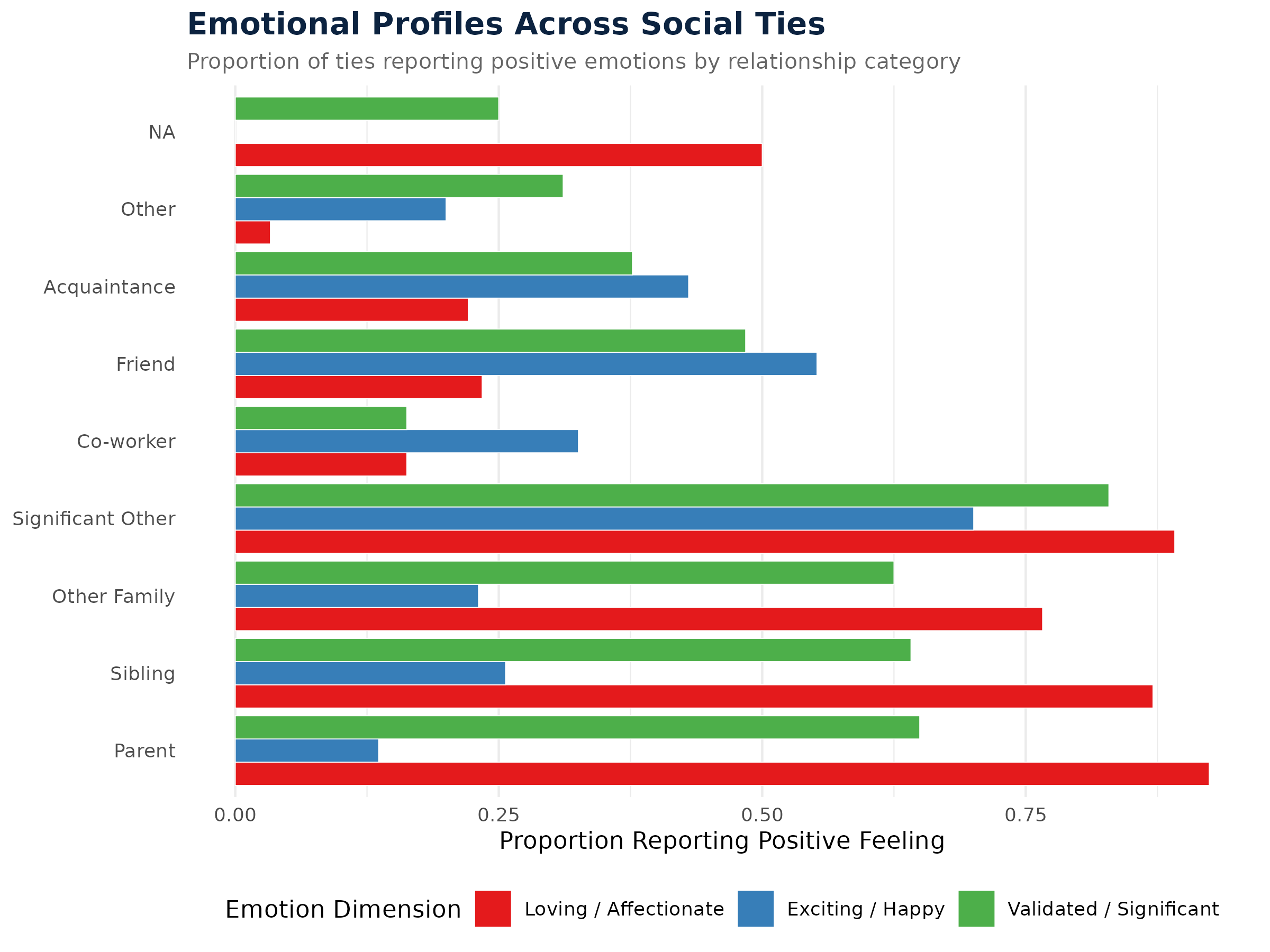
The figure below highlights the proportion of ties that are characterized by specific positive emotions (loving, exciting, or validating) across relationship types. Strong ties (romantic partners and family members) exhibit a rich emotional profile with high rates of all three dimensions.

Figure 3: Proportions of Positive Emotions Felt in Relationships

---

1.5 Perceived Alter-to-Alter Networks & Ego Metrics

In addition to direct ego-to-alter nominations, the NetSense network surveys administered an alter-by-alter matrix asking each participant whether their nominated alters knew one another:

“As far as you know, does [Alter Name] know any of your other contacts that are listed below? If you think they do, please check the boxes to indicate which of your other contacts they know. Leave boxes blank if you think [Alter Name] does not know that person.”

Originally captured across 190 conditional matrix questions per wave with wave-varying LimeSurvey naming patterns (alter{i}relsq{k}, alter{i}rel_sq{k}, and alter{i}rel{k}_sq), these variables have been parsed and structured into two standardized data files:

1. Alter-to-Alter Edge List (Data/alter_alter_ties_longitudinal.*): A dyadic edge list containing all 29,473 perceived ties between nominated alters across waves.
2. Ego-Network Structural Metrics (Data/ego_network_metrics_longitudinal.*): An ego-wave summary panel (\(N = 804\) networks) providing nominated alters (\(k\)), possible pairs (\(\binom{k}{2}\)), reported ties, and personal network density / local clustering coefficients.

1.5.1 Download Datasets

Alter-to-Alter Edge List:

Download Alter-Alter CSV (.csv) Download Alter-Alter R (.rds) Download Alter-Alter Stata (.dta)

Ego-Network Summary Metrics:

Download Ego Metrics CSV (.csv) Download Ego Metrics R (.rds) Download Ego Metrics Stata (.dta)

1.5.2 Variable Schemas & Codebook

1.5.2.1 Alter-to-Alter Edge List Schema

Variable	Type	Description
egoid	character	Primary 5-digit participant ID of the respondent (ego)
sender	character	Study survey / phone identifier of ego
wave	integer	Survey wave number (Waves 1, 2, 3, 4, 5, 7, 8)
alter1_pos	integer	Position rank of Alter 1 in ego’s nomination roster (\(1 \le \text{pos}_1 \le 19\))
alter2_pos	integer	Position rank of Alter 2 in ego’s nomination roster (\(2 \le \text{pos}_2 \le 20\))
alter1_id	character	Survey nomination identifier of Alter 1 (NA if unmapped outside alter)
alter2_id	character	Survey nomination identifier of Alter 2 (NA if unmapped outside alter)
alter1_egoid	character	5-digit participant ID if Alter 1 is a study participant (NA if non-participant)
alter2_egoid	character	5-digit participant ID if Alter 2 is a study participant (NA if non-participant)
perceived_tie	integer	Indicator (1) that ego reported Alter 1 and Alter 2 know each other

1.5.2.2 Ego-Network Metrics Schema

Variable	Type	Description
egoid	character	Primary 5-digit participant ID
sender	character	Survey identifier of ego
wave	integer	Survey wave number
alters_nominated	integer	Total nominated alters (\(k\)) in ego’s network for that wave
potential_pairs	integer	Maximum possible pairs among alters: \(\binom{k}{2} = \frac{k(k-1)}{2}\)
evaluated_pairs	integer	Total pairs evaluated in the survey matrix
perceived_ties	integer	Total count of alter-to-alter connections reported by ego
density	numeric	Alter network density / ego’s local clustering coefficient: \(\frac{\text{perceived\_ties}}{\text{potential\_pairs}}\)

1.5.3 Longitudinal Alter Network Summary by Wave

The table below summarizes ego network size, alter-alter tie counts, and average network density across all waves:

library(readr)
library(dplyr)
library(knitr)

metrics_df <- read_csv("Data/ego_network_metrics_longitudinal.csv", show_col_types = FALSE)

metrics_df |>
  group_by(Wave = wave) |>
  summarise(
    `Ego Networks` = n(),
    `Mean Alters (k)` = round(mean(alters_nominated, na.rm = TRUE), 1),
    `Total Alter Ties` = sum(perceived_ties, na.rm = TRUE),
    `Mean Alter Ties` = round(mean(perceived_ties, na.rm = TRUE), 1),
    `Mean Density` = round(mean(density, na.rm = TRUE), 3)
  ) |>
  arrange(Wave) |>
  kable(caption = "Perceived Alter-to-Alter Networks: Longitudinal Descriptives by Survey Wave")

Table 2: Perceived Alter-to-Alter Networks: Longitudinal Descriptives by Survey Wave

Wave	Ego Networks	Mean Alters (k)	Total Alter Ties	Mean Alter Ties	Mean Density
1	17	15.5	1185	69.7	0.610
2	165	14.5	7849	47.6	0.497
3	170	13.1	7390	43.5	0.536
4	123	11.6	4074	33.1	0.463
5	134	10.8	4257	31.8	0.591
7	93	9.5	2135	23.0	0.570
8	102	9.6	2583	25.3	0.602

NoteMethodological Note on Wave 6 (Summer 2013)

Perceived alter-to-alter tie data is absent for Wave 6 (Summer 2013). This is not a data loss or processing error: the alter-by-alter matrix (alter1.rel through alter19.rel) was deliberately excluded from the Wave 6 survey instrument to reduce respondent burden during the summer break (streamlining the questionnaire from 70 down to 44 items) while students were dispersed off-campus and transitioning to the junior-year study renewal. The alter-to-alter matrix battery was fully reinstated in subsequent rounds (Waves 7 and 8).