Basic Network Statistics for Directed Graphs
As we saw in the lecture notes on basic network statistics, the degree distribution and the degree correlation are two key quantities we want to understand when characterizing a network, and we showed examples for the undirected graph case. However, when you have a network measuring a tie with some meaningful “from” “to” directionality (represented as a directed graph), the number of things you have to compute in terms of degrees “doubles.”
For instance, instead of a single degree set and sequence, we now have two: an outdegree set and sequence, and an indegree set and sequence. The same thing applies to the degree distribution and the degree correlation.
Let’s see how this works. First, we load a network of directed relations represented as a directed graph. This is a network composed of advice relations between members of a low firm studied by (2001). In the networkdata package, it is called law_advice.
The nodes in this graph don’t have names, so we just assign them numbers as labels, using the graph node attribute function V(), which takes the graph object as input, followed by a $ sign and the name of the node attribute we are setting (in this case, the name attribute):
Here we set the name attribute to a vector of labels composed of “Lyr” (for lawyer) followed by a number between one and the order of the graph.
1 Graph Density
In the directed case, the formula for the density is just:
\[ d(G) = \frac{m}{n(n-1)} \tag{1}\]
Note that the main difference with the formula for undirected graphs is that we don’t double the numerator (number of edges).
So in R we would just do:
Which is the same answer we get with the igraph function edge_density:
2 Graph Reciprocity
One quantity that is only defined for directed graphs is the graph reciprocity (\(r(G)\)). This measures the extent to which directed links are mutual among actors in the network (i.e., they go both ways).
We can express the graph reciprocity in terms of the entries of the adjacency matrix \(\mathbf{A}\) as:
\[ r(G) = \sum_{i, j = 1}^N\frac{a_{ij}a_{ji}}{|E|} \tag{2}\]
Where \(|E|\) refers to the number of edges in the graph. Note that the numerator of Equation 2 counts the number of reciprocal links since the product term \(a_{ij}a_{ji}\) only when \(a_{ij}=1\) and \(a_{ji}=1\) in the adjacency matrix.
The graph reciprocity can also be expressed in “matrix” form as:
\[ r(G) = \frac{tr(\mathbf{A}^2)}{|E|} \tag{3}\]
Where \(tr\) refers to the trace matrix operation, which yields the sum of the matrix diagonal entries as a result, and the square refers to the (second) powers of the matrix (the adjacency matrix multiplied by itself).
So in R we can compute the reciprocity of a directed graph as:
[1] 0.392We use the diag function, which extracts the diagonal entries of a matrix (in this case, the square of the adjacency matrix) as a vector, and then compute the trace (the sum of the diagonal entries).
The graph reciprocity is a number between zero and one, with zero indicating that none of the connected dyads are mutual, and one indicating that all are. Of course, real networks will fall in between. As we can see, in the law advice network, about 39.2% of the observed connected dyads are composed of mutual advice relations.
Of course, there’s an igraph function to compute the graph reciprocity called (you guessed it) reciprocity:
3 Indegrees and Outdegrees
For the degree, we now have two flavors: we can count the number of nodes that point to another node (called that node’s in-neighbors), or we can count the number of nodes that a given node points to (called that node’s out-neighbors).
That means that we have two different degree vectors. The indegree vector and the outdegree vector. In igraph, we obtain those by specifying the mode argument to either in or out in the degree function:
Code
Lyr_26 Lyr_13 Lyr_17 Lyr_24 Lyr_34 Lyr_40  Lyr_2 Lyr_22  Lyr_1 Lyr_20 Lyr_21
    37     34     26     26     25     25     23     23     22     22     22
Lyr_28 Lyr_41  Lyr_6 Lyr_12 Lyr_15 Lyr_16 Lyr_30  Lyr_4 Lyr_11 Lyr_32  Lyr_5
    22     22     21     20     20     20     20     19     19     19     17
Lyr_29 Lyr_38 Lyr_39 Lyr_14 Lyr_31  Lyr_9  Lyr_8 Lyr_35 Lyr_52 Lyr_10 Lyr_18
    17     17     17     16     15     14     13     13     13     12     11
Lyr_19 Lyr_50 Lyr_57 Lyr_25 Lyr_36 Lyr_43 Lyr_56 Lyr_64 Lyr_27 Lyr_46 Lyr_49
    11     11     11     10     10     10     10     10      9      9      9
Lyr_54  Lyr_3 Lyr_23 Lyr_45 Lyr_55 Lyr_33 Lyr_60 Lyr_65  Lyr_7 Lyr_68 Lyr_70
     9      8      8      8      8      7      7      7      6      5      5
Lyr_37 Lyr_42 Lyr_48 Lyr_53 Lyr_58 Lyr_62 Lyr_67 Lyr_69 Lyr_51 Lyr_59 Lyr_63
     4      4      4      4      4      4      3      3      2      2      2
Lyr_66 Lyr_71 Lyr_47 Lyr_61 Lyr_44
     2      2      1      1      0
We can see that Lawyers 26, 13, and 17 are the most popular kids in terms of being sought after for advice.
And now for the outdegree:
Code
Lyr_19 Lyr_16 Lyr_28 Lyr_66 Lyr_42 Lyr_65 Lyr_26 Lyr_51 Lyr_24 Lyr_55 Lyr_17
    30     27     27     26     25     25     24     23     22     22     21
Lyr_27 Lyr_41 Lyr_12 Lyr_56 Lyr_31 Lyr_35  Lyr_4 Lyr_30 Lyr_33 Lyr_48 Lyr_13
    21     21     20     20     18     18     17     17     17     17     16
Lyr_67 Lyr_14 Lyr_39 Lyr_43 Lyr_54 Lyr_29 Lyr_52 Lyr_71 Lyr_22 Lyr_57 Lyr_58
    16     14     14     14     14     13     13     13     12     12     12
Lyr_60 Lyr_63 Lyr_69 Lyr_20 Lyr_21 Lyr_32 Lyr_15 Lyr_45 Lyr_50 Lyr_62 Lyr_68
    12     12     12     11     11     11     10     10     10     10     10
Lyr_23 Lyr_49 Lyr_59 Lyr_25 Lyr_40 Lyr_64  Lyr_2  Lyr_3 Lyr_10 Lyr_36 Lyr_46
     9      9      9      8      8      8      7      7      7      7      7
Lyr_70 Lyr_34 Lyr_38 Lyr_44 Lyr_11 Lyr_18 Lyr_47  Lyr_5  Lyr_7 Lyr_53  Lyr_1
     7      6      6      6      5      5      5      4      4      4      3
 Lyr_9 Lyr_37 Lyr_61  Lyr_8  Lyr_6
     3      3      3      2      0
We can see that lawyers 19, 16, and 28 are the most active advice seekers.
Just like before, we can compute various degree quantities, except we must do it twice:
[1] 892[1] 892[1] 37[1] 30[1] 0[1] 0[1] 12.56338[1] 12.56338Note that for both sum and the mean we actually don’t have to do it twice. The sum of the indegrees in a directed graph is always equal to the sum of the outdegrees, which means that the mean indegree is always equal to the mean outdegree (as that is the sum divided by the same number \(N\)).
3.1 The Indegree and Outdegree Distributions
In the case of the degree distribution, we now have two distributions: an outdegree distribution and an indegree distribution.
So the main complication is that now, just like with degree, we have to specify a value for the mode argument; in for the indegree distribution and out for the outdegree distribution.
That also means that when plotting, we have to create two data frames and present two plots.
First, the data frames:
Code
  i.d.vals     i.prop
1        0 0.01408451
2        1 0.02816901
3        2 0.07042254
4        3 0.02816901
5        4 0.08450704
6 5 0.02816901 o.d.vals o.prop
1 0 0.01408451
2 1 0.00000000
3 2 0.01408451
4 3 0.05633803
5 4 0.04225352
6 5 0.04225352Now, to plotting. To be effective, the resulting plot has to show the outdegree and indegree distributions side by side so the reader can compare them. To do that, we first generate each plot separately:
Code
library(ggplot2)
p <- ggplot(data = o.deg.dist, aes(x = o.d.vals, y = o.prop))
p <- p + geom_bar(stat = "identity", fill = "red", color = "red")
p <- p + theme_minimal()
p <- p + labs(
  x = "", y = "Proportion",
  title = "Outdegree Distribution in Law Advice Network"
)
p <- p + geom_vline(
  xintercept = mean(d.o),
  linetype = 2, linewidth = 0.75, color = "blue"
)
p1 <- p + scale_x_continuous(breaks = c(0, 5, 10, 15, 20, 25, 30, 35, 40)) + xlim(0, 40)

p <- ggplot(data = i.deg.dist, aes(x = i.d.vals, y = i.prop))
p <- p + geom_bar(stat = "identity", fill = "red", color = "red")
p <- p + theme_minimal()
p <- p + labs(
  x = "", y = "Proportion",
  title = "Indegree Distribution in Law Advice Network"
)
p <- p + geom_vline(
  xintercept = mean(d.i),
  linetype = 2, linewidth = 0.75, color = "blue"
)
p2 <- p + scale_x_continuous(breaks = c(0, 5, 10, 15, 20, 25, 30, 35, 40)) + xlim(0, 40)
Then we use the magical package patchwork to combine the plots:
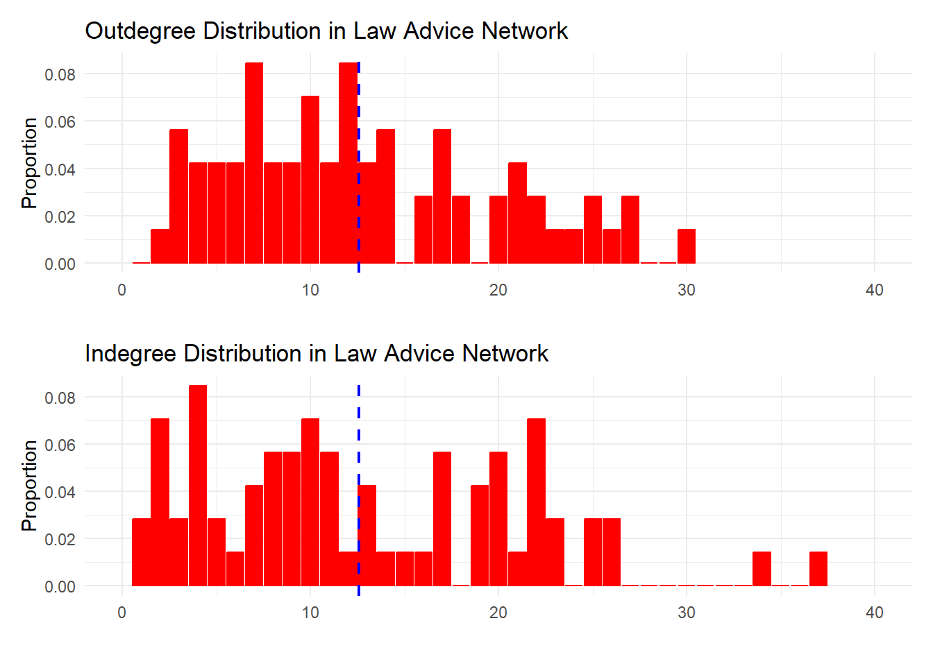
The data clearly show that, while both distributions are skewed, the indegree distribution is more heterogeneous, with a larger proportion of nodes at the high end of receiving advice than of giving advice.
Note also that, since the mean degree is the same regardless of whether we use the out- or in-degree distribution, the blue line indicating the mean degree falls at the same x-axis value in both plots.
3.2 The Four Different Flavors of Degree Correlations in the Directed Case
The same doubling (really, quadrupling) occurs for degree correlations in directed graphs. While in an undirected graph, there is a single degree correlation, in the directed case, we have four quantities to compute: The out-out degree correlation, the in-in degree correlation, the out-in degree correlation, and the in-out degree correlation (see here, p. 38).
To proceed, we need to create an edge list data set with six columns: The node ID of the “from” node, the node ID of the “to” node, the indegree of the “from” node, the outdegree of the “from” node, the indegree of the “to” node, and the outdegree of the “to” node.
We can adapt the code we used for the undirected case for this purpose. First, we create an edge list data frame using the igraph function as_long_data_frame, specifying that we only want the columns that have the names of the respective nodes incident to the edge:
Code
     fr     to
1 Lyr_1  Lyr_2
2 Lyr_1 Lyr_17
3 Lyr_1 Lyr_20
4 Lyr_2  Lyr_1
5 Lyr_2  Lyr_6
6 Lyr_2 Lyr_17
Second, we create data frames containing the in and outdegrees of each node in the network:
Third, we merge this info into the edge list data frame to get the in and outdegrees of the from and to nodes in the directed edge:
Code
     fr     to d.o.fr d.i.fr d.o.to d.i.to
1 Lyr_1  Lyr_2      3     22      7     23
2 Lyr_1 Lyr_17      3     22     21     26
3 Lyr_1 Lyr_20      3     22     11     22
4 Lyr_2  Lyr_1      7     23      3     22
5 Lyr_2  Lyr_6      7     23      0     21
6 Lyr_2 Lyr_17      7     23     21     26
Now we can compute the four different flavors of the degree correlation for directed graphs:
[1] -0.0054[1] 0.187[1] -0.0283[1] -0.0843These results tell us that there is not much degree assortativity going on in the law advice network, except for a slight tendency of people who receive advice from lots of others to give advice to people who also receive advice from a lot of other people (the “in-in” correlation)
Note that by default, the assortativity_degree function in igraph only returns the out-in correlation for directed graphs:
That is, assortativity_degree checks if more active senders are more likely to send ties to people who are popular receivers of ties.