   link.bag <- function(x, c) {
      library(dplyr)
      g.el <- data.frame(as_edgelist(x))
      names(g.el) <- c("vi", "vj")
      comm.dat <- data.frame(vi = as.vector(V(x)),
                             vj = as.vector(V(x)),
                             c = as.vector(c))
      el.temp <- data.frame(vj = g.el[, 2]) %>%
         left_join(comm.dat, by = "vj") %>%
         dplyr::select(c("vj", "c")) %>%
         rename(c2 = c)
      d.el <- data.frame(vi = g.el[, 1]) %>%
         left_join(comm.dat, by = "vi") %>%
         dplyr::select(c("vi", "c")) %>%
         rename(c1 = c) %>%
         cbind(el.temp)
   return(d.el)
}Community Structure
What are communities?
What are communities? In networks, communities are subsets of nodes that have more interactions or connectivity within themselves than outside of themselves (these are sometimes called “modules” outside sociology). Communities thus exemplify the sociological concept of a group.
A network has community structure if it contains many such subsets or groups of nodes that interact preferentially with one another. Not all networks have to have community structure; a network in which all nodes interact with equal propensity doesn’t have communities.
So whether a network has community structure, and whether a given guess about what these communities are yields actual communities (a cluster of nodes that interact more among themselves than with outsiders) is an empirical question that needs to be answered with data.
But first, we need to develop a criterion for determining whether a given partition of the network into mutually exclusive node subsets actually produces communities as we defined them earlier. This criterion should be independent of particular methods and algorithms that claim to find communities, so that we can compare them with one another and see whether the partitions they recommend yield actual communities.
Mark Newman (2006b), who has done the most influential work in this area, proposed such a criterion and called it the modularity of a partition (e.g., the extent to which a partition has identified the “modules” or subsets of the network).
A bag of links
An intuitive way to understand the modularity is as follows. Imagine we have an idea of what the communities in a network are. This could be given by a special community partitioning method, our intuition, or exogenous node coloring (e.g., based on a node attribute such as race, gender, or position in the organization). The membership of each node in each community is thus stored in a vector, \(C_i = k\) if node \(i\) belongs to community \(k\); this vector is of length \(N\) where \(N\) is the number of nodes in the network.
Our job is to decide whether that community partition is good, in the sense of dividing the nodes into subsets that interact preferentially with one another and not with outsiders.
One way to proceed is to imagine that we take the network in question, and we throw each observed link into a bag. Then our modularity measure should give us an idea of the probability that, if we drew a link at random, the nodes at its ends belong to the same community (or have the same color if the communities are defined by exogenous attributes). If the probability is high, then the network has a community structure. If the probability is no better than we would expect under a null model that assumes nothing is going on in the network connectivity-wise except random chance, then the modularity should be low (and we decide that the partition we chose does not divide the network into meaningful communities).
Let’s assume our bag of links contains only directed links, and we draw a bunch of them at random. Let’s call the node at the starting end of the link \(s\) and the node at the destination end of the link \(d\). Then we can measure the modularity—let’s call it \(Q\)—of a given partition of the network into \(m\) clusters as follows:
\[ Q = \sum_{k = 1}^m \left[P(s \in k \land d \in k) - P(s \in k) \times P(d \in k) \right] \]
In this equation, \(P(s \in k \land d \in k)\) is the probability that a link drawn at random has a source and a destination node that belong to the same community \(k\); \(P(s \in k)\) is just the probability of drawing a link that has a starting node in community \(k\) (regardless of the membership of the destination node) and \(P(d \in k)\) is the probability of drawing a link that has a destination node that belongs to community \(k\) (regardless of the membership fo the source node).
If you remember your elementary probability theory, you know that the joint probability of two events that are assumed to be independent of one another is just the product of their individual probabilities. So that means that \(P(s \in k) \times P(d \in k)\) is the expected probability of finding that both the source and destination node are in the same community \(k\) in a network in which communities don’t matter for link formation (because the two probabilities are assumed to be independent).
So the formula for the modularity subtracts the observed probability of finding links with two nodes in the same community from what we would expect if communities didn’t matter. So it measures the extent to which we find within-community links in the network beyond what we would expect by chance. Obviously, the higher this number, the higher the deviation from chance is, and the more community structure there is in the network.
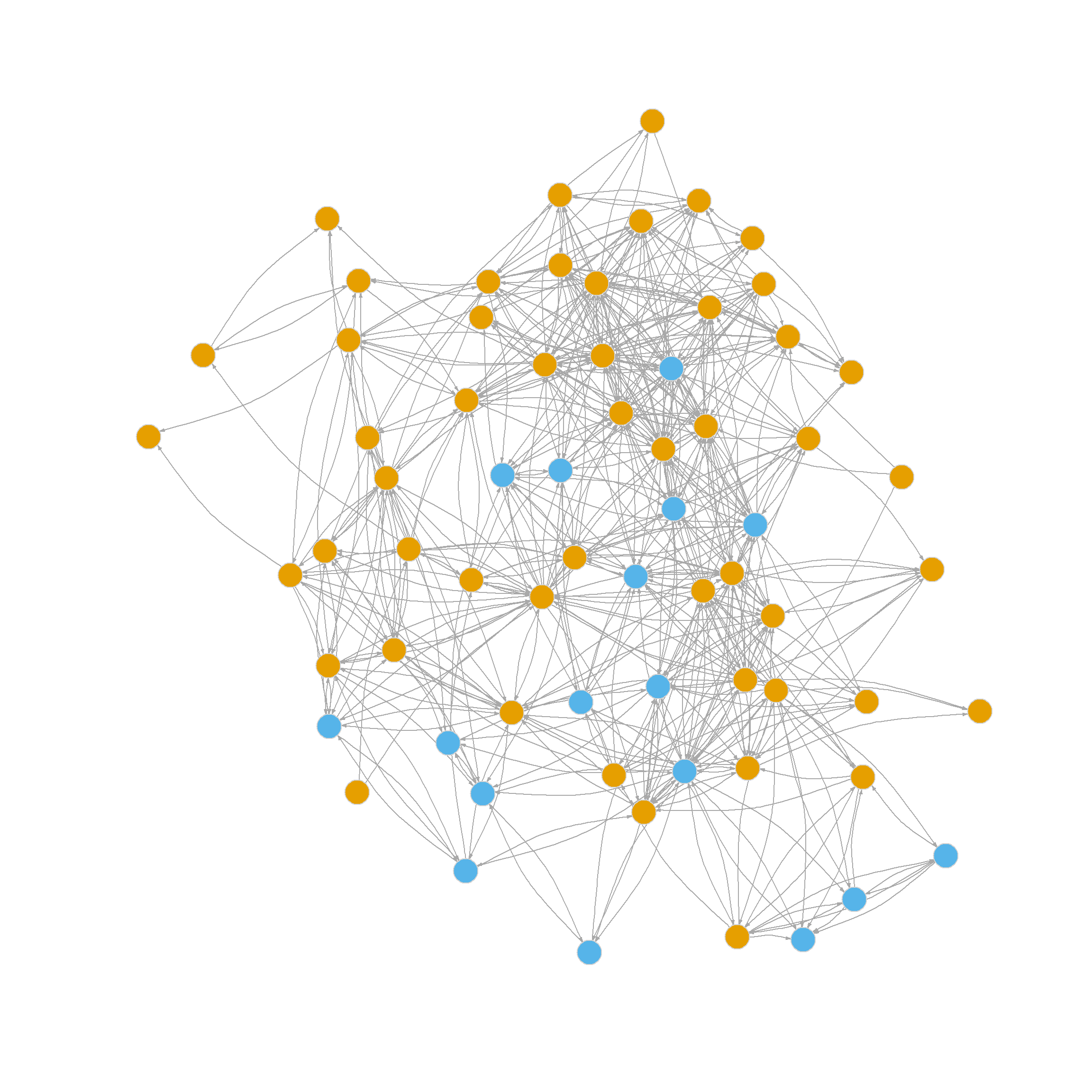
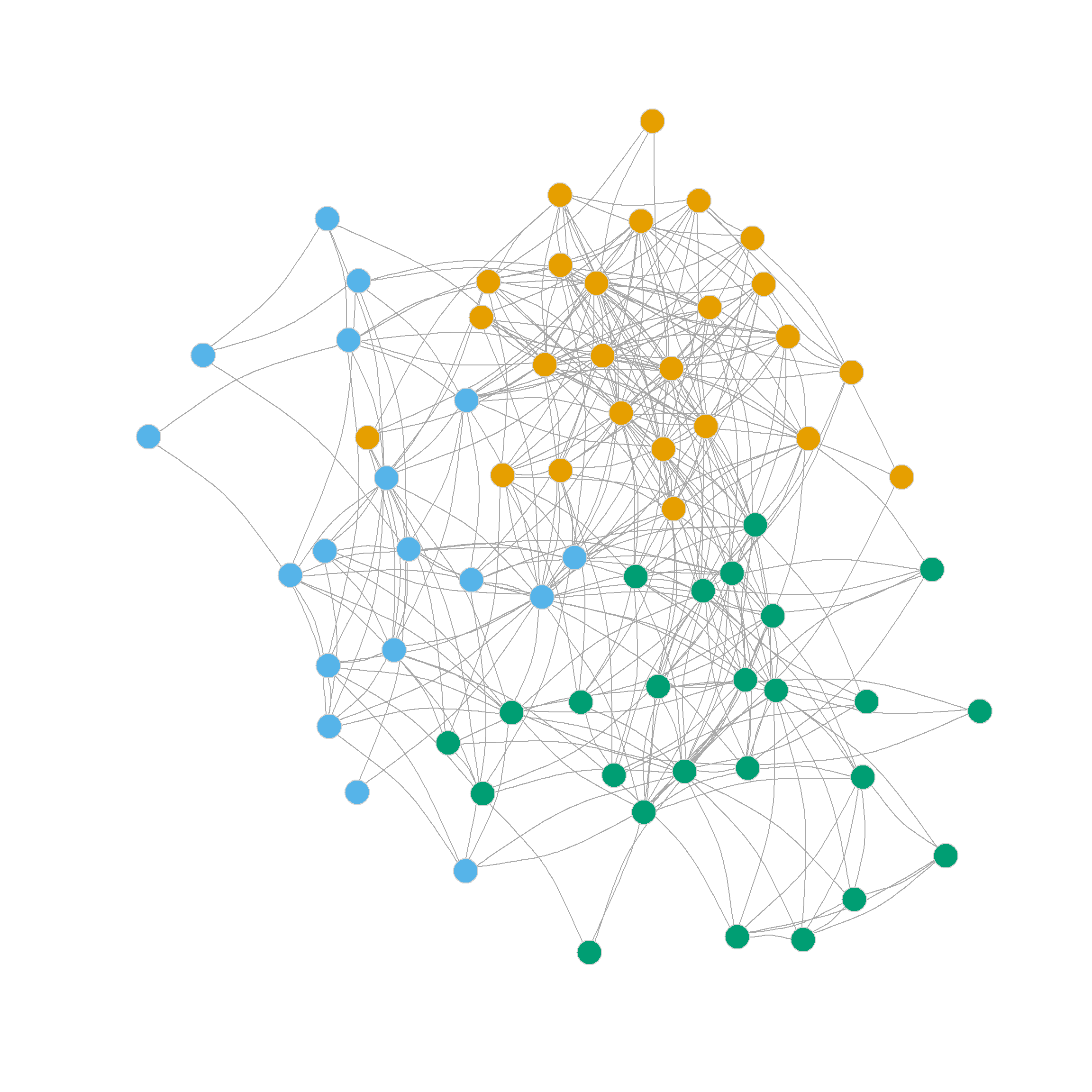
Let’s move to a real example. Figure 1 shows two plots of the friendship nomination network from the law_friends data (Lazega 2001) from the networkdata package (dropping nodes that have a degree of one). The first shows nodes colored by status within the firm (partners in tan, associates in blue), and the other shows nodes colored by gender (men in tan, women in blue).
It is pretty evident that there is more community partitioning in the network by status than by gender; that is, friendship nominations tend to go from people of a given rank to people of the same rank, which makes sense. So a measure of modularity should be higher when using status as our partition than when using gender.

Let’s see an example of the modularity computed using our “bag of links” framework. Below is a quick function that uses dplyr to take a graph as input and return an edge list data frame containing the “community membership” of each node for the characteristic specified by the second input.
So if we wanted an edge list data frame containing each node’s status membership in the law_advice network, we would just type:
  vi c1 vj c2
1  1  1  2  1
2  1  1  4  1
3  1  1  8  1
4  1  1 17  1
5  2  1 16  1
6  2  1 17  1
Note that an edge list is already a “bag of links,” so we can obtain the three probabilities we need to compute the modularity of a partition directly from the edge list data frame. Here’s a function that does this:
   mod.Q1 <- function(x, c1 = 2, c2 = 4) {
      Q <- 0
      comms <- unique(x[, c1])
      for (k in comms) {
         e.same <- x[x[, c1] == k & x[, c2] == k, ]
         e.sour <- x[x[, c1] == k, ]
         e.dest <- x[x[, c2] == k, ]
         e.total <- nrow(x)
         p.same <- nrow(e.same)/e.total
         p.sour <- nrow(e.sour)/e.total
         p.dest <- nrow(e.dest)/e.total
         Q <- Q + (p.same - (p.sour * p.dest))
      }
   return(Q)
   }
This function takes the edge list data frame as input. Optionally, you can specify the two columns containing community membership info for the source and destination nodes in each link (in this case, the second and fourth columns). The Function works like this:
The probability of a link drawn randomly from the bag is just the number of links where the source and destination links belong to the same community (
e.same, computed in line 5) divided by the total number of links (which is the number of rows in the edge list data frame), this ratio is computed in line 9 (p.same).The overall probability of a link containing a source node in community \(k\) is computed in line 10 (
p.sour), and the overall probability of a link containing a destination node in community \(k\) is computed in line 11 (p.dest).The actual modularity is computed step by step by summation across levels of the community indicator variable in line 12, which is the sum of the difference between
p.sameand the product ofp.sourtimesp.destacross all communities \(m\) (in this case \(m = 2\) as there are only two levels of status).
So if we wanted to check if status was more powerful in structuring the community organization of the law_friends network than gender, we would just type:
This indeed confirms that status is a more powerful group formation principle than gender in this network.
Modularity from the Adjacency Matrix
Note that while the “bag of links” idea is useful for illustrating the basic probabilistic principle behind modularity in a network, we can compute it directly from the adjacency matrix without going through the edge-list data-frame construction step.
A function that does this looks like:
This function takes a graph and a vector indicating each node’s community membership and returns the modularity. Like before the modularity is the difference in the probability of observing a within-community link between two nodes (given by the ratio of the number of links in the sub-adjacency matrix containing only within community-nodes—obtained in line 7—and the overall number of links in the adjacency matrix, computed in line 3) and the expected probability of a link between a source node with community membership \(k\) and a destination node with the same community membership.
This last quantity is given by the product of the sum links in a the sub-adjacency matrix with row nodes that belong to community \(k\) (the source nodes) and the number of links in the sub adjacency matrix with the column nodes belonging to community \(k\) (the destination nodes) divided by the square of the total number of links observed the network.
In formulese:
\[\begin{equation} Q = \sum_{k=1}^m \left[\frac{\sum_{i \in k} \sum_{j \in k} a_{ij}}{\sum_i \sum_j a_{ij}} - \frac{(\sum_{i \in k} \sum_j a_{ij})(\sum_i \sum_{j \in k} a_{ij})}{(\sum_i \sum_j a_{ij})^2} \right] \end{equation}\]
Where \(\sum_i \sum_ja_{ij}\) is the sum of all the entries in the network adjacency matrix, \(\sum_{i \in k} \sum_{j \in k} a_{ij}\) is the sum of all the entries of the sub-adjacency matrix where both the row and column nodes come from community \(k\), \(\sum_{i \in k} \sum_j a_{ij}\) is the sum of all the entries in the sub-adjacency matrix where only the row nodes come from community \(k\), and \(\sum_i \sum_{j \in k} a_{ij}\) is the sum of all the entries in the sub-adjacency matrix where only the column nodes come from community \(k\).
We can easily see that this approach gives us the same answer as the bag of links version:
Of course, you don’t even have to use a custom function like the above, because igraph has one, called (you guessed it) modularity:
But at least now you know what’s going on inside of it!
The Modularity Matrix
Obviously, modularity wouldn’t be widely used if it were merely a way to measure the quality of a community partition produced by other methods. It can be used to find community partitions by a method that produces a node partition capturing the largest values it can take in a graph.
A useful tool in this quest is the modularity matrix \(\mathbf{B}\) (Newman 2006b), which is defined as a variation on the adjacency matrix \(\mathbf{A}\), where each cell of the modularity matrix \(b_{ij}\) takes the value:
\[ b_{ij} = a_{ij} - \frac{k^{out}_ik^{in}_j}{\sum_i\sum_j a_{ij}} \]
Where \(k^{out}_i\) is node \(i\)’s outdegree and \(k^{in}_j\) is node j’s indegree. Note that the modularity matrix has the same “observed minus expected” structure as the formulas for the modularity. In this case, we compare whether we see a link from \(i\) to \(j\) as given by \(a_{ij}\) against the chances of observing a link in a graph in which nodes connect at random with probability proportional to their degrees (as given by the right-hand side fraction).
Note that if the graph is undirected, the modularity matrix is just:
\[ b_{ij} = a_{ij} - \frac{k_ik_j}{\sum_i\sum_j a_{ij}} \]
A function to compute the modularity matrix by looping through every element of the adjacency matrix for a directed graph looks like:
Peeking inside the resulting matrix:
        [,1]   [,2]   [,3]   [,4]   [,5]   [,6]   [,7]   [,8]   [,9]  [,10]
 [1,] -0.035  0.930 -0.028  0.902 -0.035 -0.014 -0.014  0.951 -0.098 -0.028
 [2,] -0.035 -0.070 -0.028 -0.098 -0.035 -0.014 -0.014 -0.049 -0.098 -0.028
 [3,]  0.000  0.000  0.000  0.000  0.000  0.000  0.000  0.000  0.000  0.000
 [4,] -0.131  0.739  0.895 -0.366 -0.131 -0.052 -0.052 -0.183  0.634 -0.105
 [5,] -0.026 -0.052 -0.021 -0.073 -0.026 -0.010  0.990 -0.037 -0.073 -0.021
 [6,]  0.000  0.000  0.000  0.000  0.000  0.000  0.000  0.000  0.000  0.000
 [7,] -0.017 -0.035  0.986 -0.049  0.983 -0.007 -0.007 -0.024 -0.049 -0.014
 [8,] -0.009 -0.017 -0.007 -0.024 -0.009 -0.003 -0.003 -0.012 -0.024 -0.007
 [9,] -0.052 -0.105 -0.042  0.854 -0.052 -0.021 -0.021 -0.073 -0.146 -0.042
[10,] -0.122  0.756 -0.098 -0.341 -0.122 -0.049 -0.049  0.829  0.659 -0.098
Interestingly, the matrix has some negative entries, some positive entries, and some close to or actually zero. We interpret these as follows: If an entry is negative, it means that a link between the row and column nodes is much less likely to happen than expected given each node’s degrees, a positive entry indicates the opposite; a larger than expected chance of a link forming. Entries close to zero indicate those nodes have odds close to a random chance of forming a tie.
Of course, igraph has a function, called modularity_matrix, which gives us the same result:
        [,1]   [,2]   [,3]   [,4]   [,5]   [,6]   [,7]   [,8]   [,9]  [,10]
 [1,] -0.035  0.930 -0.028  0.902 -0.035 -0.014 -0.014  0.951 -0.098 -0.028
 [2,] -0.035 -0.070 -0.028 -0.098 -0.035 -0.014 -0.014 -0.049 -0.098 -0.028
 [3,]  0.000  0.000  0.000  0.000  0.000  0.000  0.000  0.000  0.000  0.000
 [4,] -0.131  0.739  0.895 -0.366 -0.131 -0.052 -0.052 -0.183  0.634 -0.105
 [5,] -0.026 -0.052 -0.021 -0.073 -0.026 -0.010  0.990 -0.037 -0.073 -0.021
 [6,]  0.000  0.000  0.000  0.000  0.000  0.000  0.000  0.000  0.000  0.000
 [7,] -0.017 -0.035  0.986 -0.049  0.983 -0.007 -0.007 -0.024 -0.049 -0.014
 [8,] -0.009 -0.017 -0.007 -0.024 -0.009 -0.003 -0.003 -0.012 -0.024 -0.007
 [9,] -0.052 -0.105 -0.042  0.854 -0.052 -0.021 -0.021 -0.073 -0.146 -0.042
[10,] -0.122  0.756 -0.098 -0.341 -0.122 -0.049 -0.049  0.829  0.659 -0.098
In the case of an undirected graph, computing the modularity is even simpler:
Let’s see the function in action:
       [,1]  [,2]  [,3]  [,4]  [,5]  [,6]  [,7]  [,8]  [,9] [,10]
 [1,] -0.08  0.90 -0.04  0.78 -0.06 -0.02 -0.03  0.93 -0.14 -0.14
 [2,]  0.90 -0.13 -0.05  0.72 -0.08 -0.03 -0.04 -0.09 -0.18  0.82
 [3,] -0.04 -0.05 -0.02  0.89 -0.03 -0.01  0.98 -0.04 -0.07 -0.07
 [4,]  0.78  0.72  0.89 -0.61 -0.17 -0.06 -0.08 -0.19  0.61 -0.39
 [5,] -0.06 -0.08 -0.03 -0.17 -0.05 -0.02  0.98 -0.05 -0.11 -0.11
 [6,] -0.02 -0.03 -0.01 -0.06 -0.02 -0.01 -0.01 -0.02 -0.04 -0.04
 [7,] -0.03 -0.04  0.98 -0.08  0.98 -0.01 -0.01 -0.03 -0.05 -0.05
 [8,]  0.93 -0.09 -0.04 -0.19 -0.05 -0.02 -0.03 -0.06 -0.12  0.88
 [9,] -0.14 -0.18 -0.07  0.61 -0.11 -0.04 -0.05 -0.12 -0.25  0.75
[10,] -0.14  0.82 -0.07 -0.39 -0.11 -0.04 -0.05  0.88  0.75 -0.25
Which gives us the same results as using igraph:
       [,1]  [,2]  [,3]  [,4]  [,5]  [,6]  [,7]  [,8]  [,9] [,10]
 [1,] -0.08  0.90 -0.04  0.78 -0.06 -0.02 -0.03  0.93 -0.14 -0.14
 [2,]  0.90 -0.13 -0.05  0.72 -0.08 -0.03 -0.04 -0.09 -0.18  0.82
 [3,] -0.04 -0.05 -0.02  0.89 -0.03 -0.01  0.98 -0.04 -0.07 -0.07
 [4,]  0.78  0.72  0.89 -0.61 -0.17 -0.06 -0.08 -0.19  0.61 -0.39
 [5,] -0.06 -0.08 -0.03 -0.17 -0.05 -0.02  0.98 -0.05 -0.11 -0.11
 [6,] -0.02 -0.03 -0.01 -0.06 -0.02 -0.01 -0.01 -0.02 -0.04 -0.04
 [7,] -0.03 -0.04  0.98 -0.08  0.98 -0.01 -0.01 -0.03 -0.05 -0.05
 [8,]  0.93 -0.09 -0.04 -0.19 -0.05 -0.02 -0.03 -0.06 -0.12  0.88
 [9,] -0.14 -0.18 -0.07  0.61 -0.11 -0.04 -0.05 -0.12 -0.25  0.75
[10,] -0.14  0.82 -0.07 -0.39 -0.11 -0.04 -0.05  0.88  0.75 -0.25
The modularity matrix has some interesting properties. For instance, both its rows and columns sum to zero:
 [1] 0 0 0 0 0 0 0 0 0 0 0 0 0 0 0 0 0 0 0 0 0 0 0 0 0 0 0 0 0 0 0 0 0 0 0 0 0 0
[39] 0 0 0 0 0 0 0 0 0 0 0 0 0 0 0 0 0 0 0 0 0 0 0 0 0 0 0 0 0 0 [1] 0 0 0 0 0 0 0 0 0 0 0 0 0 0 0 0 0 0 0 0 0 0 0 0 0 0 0 0 0 0 0 0 0 0 0 0 0 0
[39] 0 0 0 0 0 0 0 0 0 0 0 0 0 0 0 0 0 0 0 0 0 0 0 0 0 0 0 0 0 0Which makes \(\mathbf{B}\) doubly centered a neat but so far useless property.
Using the Modularity Matrix to Find the Modularity of a Partition
A more interesting property of the modularity matrix is that we can use it to compute the actual modularity of a given binary partition of the network into clusters. Let’s take status in the law_friends network as an example.
First, we create a new vector \(\mathbf{s}\) that equals one when node \(i\) is in the first group (partners) and minus one when node \(i\) is in the second group (associates):
 [1]  1  1  1  1  1  1  1  1  1  1  1  1  1  1  1  1  1  1  1  1  1  1  1  1  1
[26]  1  1  1  1  1  1  1  1  1  1  1 -1 -1 -1 -1 -1 -1 -1 -1 -1 -1 -1 -1 -1 -1
[51] -1 -1 -1 -1 -1 -1 -1 -1 -1 -1 -1 -1 -1 -1 -1 -1 -1 -1
Once we have this vector, the modularity is just:
\[ Q = \frac{\mathbf{s}^T\mathbf{B}\mathbf{s}}{2\sum_i\sum_ja_{ij}} \]
Which we can readily check in R:
You can think of the \(\mathbf{s}\) vector as identifying the binary community membership via contrast coding.
We can also use the modularity matrix to find the modularity of a partition via dummy coding. To do this, we create two vectors for each level of the group membership variable with \(u^{(1)}_i = 1\) when when node \(i\) is a partner (otherwise \(u^{(1)}_i = 0\)), and \(u^{(2)}_i = 1\) when when node \(i\) is an associate (otherwise \(u^{(2)}_i = 0\)).
In R, we can do this as follows:
We then join the two vectors into a matrix \(\mathbf{U}\) of dimensions \(n \times 2\):
     u1 u2
[1,]  1  0
[2,]  1  0
[3,]  1  0
[4,]  1  0
[5,]  1  0
[6,] 1 0 u1 u2
[63,] 0 1
[64,] 0 1
[65,] 0 1
[66,] 0 1
[67,] 0 1
[68,] 0 1Once we have this matrix, the modularity of the partition is given by:
\[ \frac{tr(U^TBU)}{\sum_i\sum_ja_{ij}} \]
Where \(tr\) denotes the trace operation in a matrix, namely, taking the sum of its diagonal elements.
We can check that this gives us the correct solution in R as follows:
Neat! It makes sense (given the name of the matrix) that we can compute the modularity from \(\mathbf{B}\), and we can do it in multiple ways.
Using the Modularity Matrix to Find Communities
Here’s an even more useful property of the modularity matrix. Remember the network distribution game we played to define our various reflective status measures in our discussion of prestige?
   status1 <- function(w) {
      x <- rep(1, nrow(w)) #initial status vector set to all ones of length equal to the number of nodes
      d <- 1 #initial delta
      k <- 0 #initializing counter
      while (d > 1e-10) {
          o.x <- x #old status scores
          x <- w %*% o.x #new scores are a function of old scores and adjacency matrix
          x <- x/norm(x, type = "E") #normalizing new status scores
          d <- abs(sum(abs(x) - abs(o.x))) #delta between new and old scores
          k <- k + 1 #incrementing while counter
      }
   return(as.vector(x))
   }
What if we played it with the modularity matrix?
 [1] -0.10 -0.14 -0.02 -0.21 -0.03  0.00  0.01 -0.05 -0.21 -0.18 -0.16 -0.24
[13] -0.13 -0.06 -0.04 -0.12 -0.24  0.08 -0.03 -0.17 -0.18 -0.15 -0.09 -0.14
[25] -0.11 -0.17 -0.19  0.04 -0.10 -0.02  0.11  0.06  0.06 -0.06  0.10  0.01
[37] -0.05  0.04 -0.05  0.12  0.19 -0.02  0.07  0.05  0.02  0.08  0.08  0.09
[49]  0.17  0.00  0.20  0.06  0.20  0.13  0.20  0.09  0.08  0.05  0.06  0.02
[61]  0.24  0.14  0.17  0.06  0.13  0.09  0.09  0.09
This seems more interesting. The resulting “status” vector has both negative and positive entries. What if I told you that this vector is actually a partition of the original graph into two communities?
Not only that, I have even better news. This is the partition that maximizes the modularity in the graph, the best two-group partition that has the most edges within groups and the least edges going across groups.1
Let’s see some evidence for these claims in real data.
First, let’s turn the “status” vector into a community indicator vector. We assign all nodes with scores larger than zero to one community and nodes with scores equal to zero or less to the other one:
 1  2  3  4  5  6  7  8  9 10 11 12 13 14 15 16 17 18 19 20 21 22 23 24 25 26
 1  1  1  1  1  2  2  1  1  1  1  1  1  1  1  1  1  2  1  1  1  1  1  1  1  1
27 28 29 30 31 32 33 34 35 36 37 38 39 40 41 42 43 44 45 46 47 48 49 50 51 52
 1  2  1  1  2  2  2  1  2  2  1  2  1  2  2  1  2  2  2  2  2  2  2  2  2  2
53 54 55 56 57 58 59 60 61 62 63 64 65 66 67 68
 2  2  2  2  2  2  2  2  2  2  2  2  2  2  2  2
And for the big check:
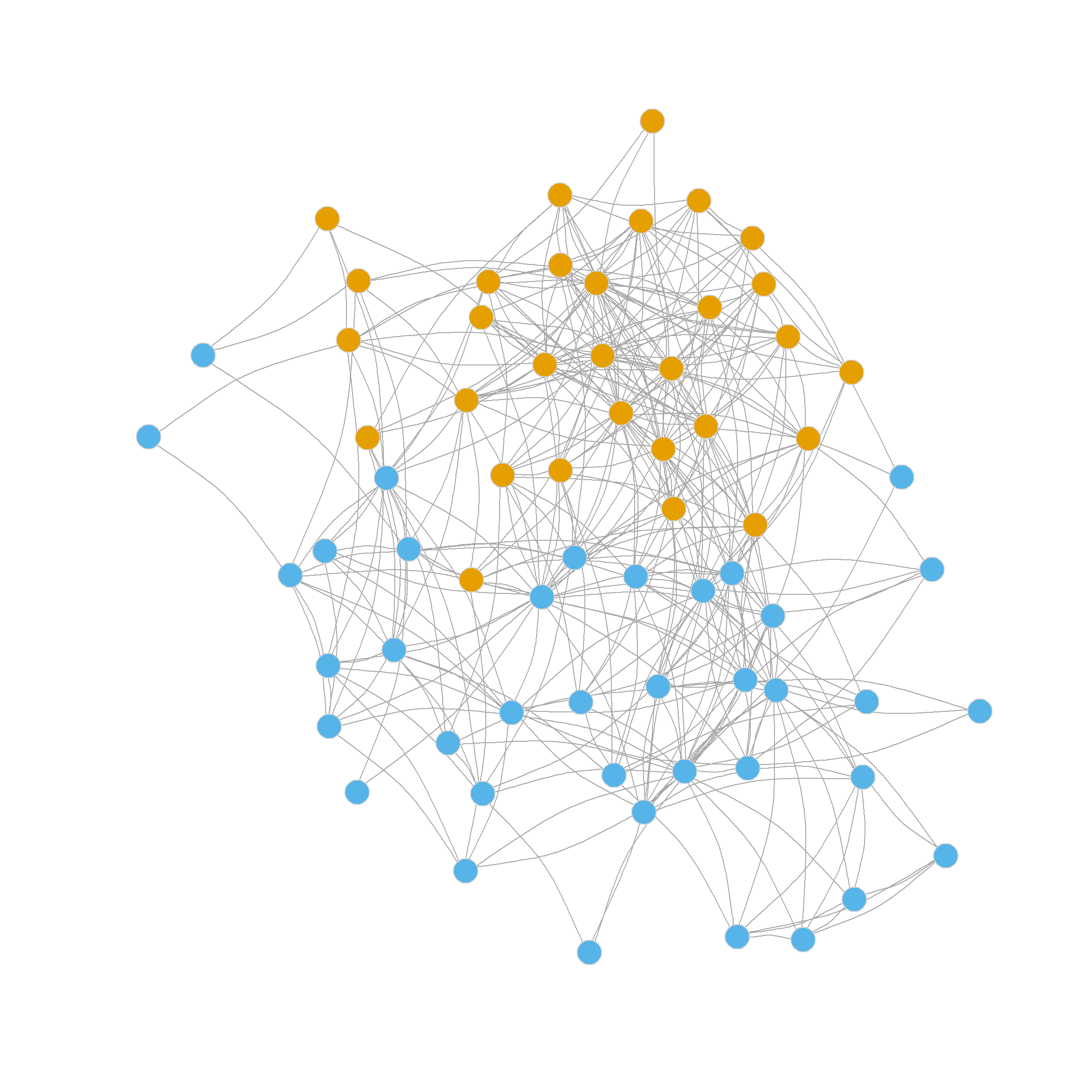
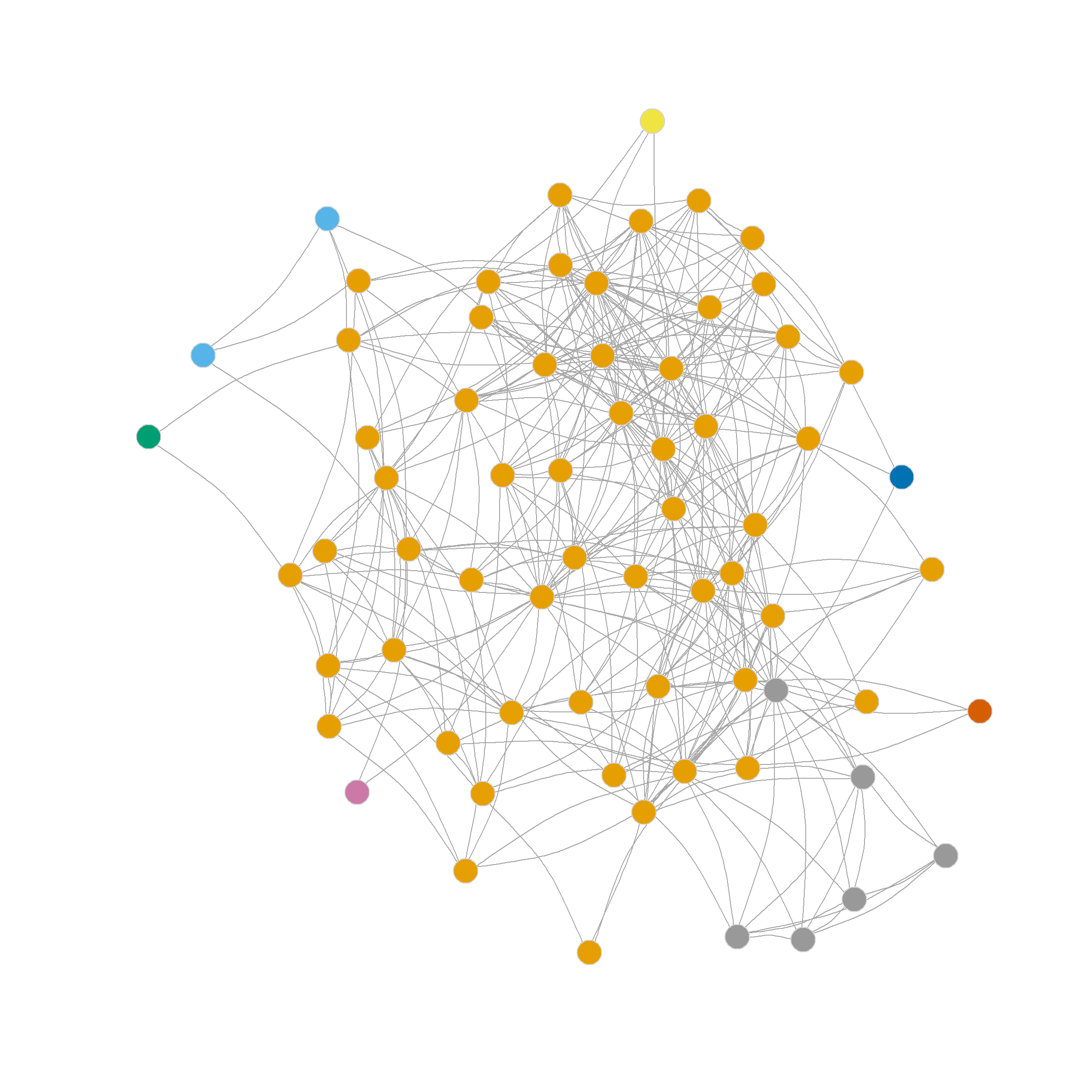
This is a pretty big score, at least larger than we obtained earlier using the exogenous indicator of status in the law firm as the basis for a binary partition. Figure 2 shows visual evidence that this is indeed an optimal binary partition of the law_friends network.
Of course, you may also remember from the Status and Prestige lesson that the little status game we played above is also a method (called the “power” method) of computing the leading eigenvector (the one associated with the largest eigenvalue) of a matrix. So turns out that the modularity maximizing bi-partition of a graph is just given by this vector:
\[ \mathbf{B}\mathbf{v} = \lambda\mathbf{v} \]
Solving for \(\mathbf{v}\) in the equation above yields the nodes’ community memberships. In R, you can do this using the native eigen function as we did for the status scores:
 [1] -0.10 -0.14 -0.02 -0.21 -0.03  0.00  0.01 -0.05 -0.21 -0.18 -0.16 -0.24
[13] -0.13 -0.06 -0.04 -0.12 -0.24  0.08 -0.03 -0.17 -0.18 -0.15 -0.09 -0.14
[25] -0.11 -0.17 -0.19  0.04 -0.10 -0.02  0.11  0.06  0.06 -0.06  0.10  0.01
[37] -0.05  0.04 -0.05  0.12  0.19 -0.02  0.07  0.05  0.02  0.08  0.08  0.09
[49]  0.17  0.00  0.20  0.06  0.20  0.13  0.20  0.09  0.08  0.05  0.06  0.02
[61]  0.24  0.14  0.17  0.06  0.13  0.09  0.09  0.09
Which look like the same values we obtained earlier.
We can package all of the steps above into a simple function:
And check to see if it works:
 1  2  3  4  5  6  7  8  9 10 11 12 13 14 15 16 17 18 19 20 21 22 23 24 25 26
 1  1  1  1  1  2  2  1  1  1  1  1  1  1  1  1  1  2  1  1  1  1  1  1  1  1
27 28 29 30 31 32 33 34 35 36 37 38 39 40 41 42 43 44 45 46 47 48 49 50 51 52
 1  2  1  1  2  2  2  1  2  2  1  2  1  2  2  1  2  2  2  2  2  2  2  2  2  2
53 54 55 56 57 58 59 60 61 62 63 64 65 66 67 68
 2  2  2  2  2  2  2  2  2  2  2  2  2  2  2  2
Indeed, it splits the nodes in a graph into two modularity-maximizing communities.
It is clear that this approach hints at a divisive partitioning strategy, where we begin with two communities and then try to split one (or both) of those communities into two more, as with CONCOR.
However, unlike CONCOR, we don’t want to be unprincipled here because splitting a well-defined community into two just for the hell of it can actually lead to worse modularity than keeping the original larger communities.
So we need an approach that tries out splitting one of the original two communities into two smaller ones, checks the new modularity, compares it with the old, and only proceeds with the partition if the new modularity is greater than the old.
Here’s one way of doing that:
   split.mult <- function(B, vol, u, v, s = 0.01) {
      split <- list()
      delta.Q <- rep(0, max(v))
      for (i in 1:max(v)) {
         old.Q <- t(u[, i]) %*% B %*% u[, i] #Using dummy coding to compute Q
         sub <- which(u[, i] == 1)
         new.B <- B[sub, sub]
         new.u <- split.two(new.B)$dummy
         new.v <- split.two(new.B)$v
         Q1 <- t(new.u[, 1]) %*% new.B %*% new.u[, 1] #Using dummy coding to compute Q
         Q2 <- t(new.u[, 2]) %*% new.B %*% new.u[, 2] #Using dummy coding to compute Q
         new.Q <- Q1 + Q2
         delta.Q[i] <- (new.Q - old.Q) * (1/vol)
         if (delta.Q[i] > s) {
            split[[i]] <- new.v
            names(split[[i]]) <- which(u[, i] == 1)
            }
         else if (delta.Q[i] <= s) {
            split[[i]] <- NULL
            }
      }
   return(list(delta.Q = round(delta.Q, 3), v = v, split = split))
   }
This function uses the output of the split.two function to check whether either of the two sub-communities should be split into two further sub-communities by comparing the modularities pre- and post-second partition.
Here are the results applied to the law_friends network:
   s <- split.mult(B = Bu,
                   vol = sum(as.matrix(as_adjacency_matrix(ug))),
                   u = split.two(Bu)$dummy,
                   v = split.two(Bu)$v)
   s
$delta.Q
[1] 0.000 0.048
$v
1 2 3 4 5 6 7 8 9 10 11 12 13 14 15 16 17 18 19 20 21 22 23 24 25 26
1 1 1 1 1 2 2 1 1 1 1 1 1 1 1 1 1 2 1 1 1 1 1 1 1 1
27 28 29 30 31 32 33 34 35 36 37 38 39 40 41 42 43 44 45 46 47 48 49 50 51 52
1 2 1 1 2 2 2 1 2 2 1 2 1 2 2 1 2 2 2 2 2 2 2 2 2 2
53 54 55 56 57 58 59 60 61 62 63 64 65 66 67 68
2 2 2 2 2 2 2 2 2 2 2 2 2 2 2 2
$split
$split[[1]]
NULL
$split[[2]]
6 7 18 28 31 32 33 35 36 38 40 41 43 44 45 46 47 48 49 50 51 52 53 54 55 56
2 2 2 2 2 2 2 2 2 1 1 1 1 1 1 1 2 2 1 1 1 1 1 1 2 2
57 58 59 60 61 62 63 64 65 66 67 68
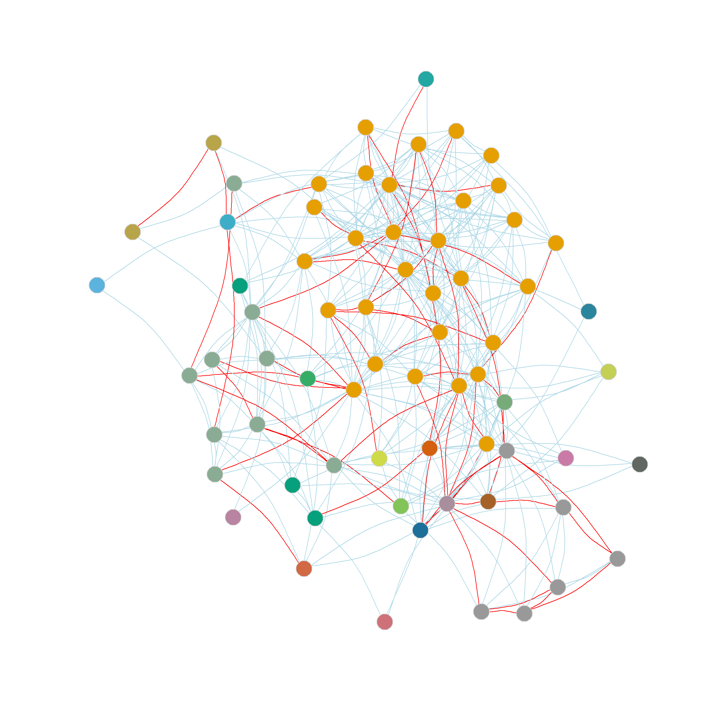
2 1 1 2 1 1 1 1 1 1 1 1 The delta.Q vector stores the results of our modularity checks. In this case, the test in the first community failed; the modularity didn’t change (the difference between the old and the new is zero) when we tried to split into two smaller communities. This is usually indicative that the original community was a well-defined group with lots of within-cluster ties, so that splitting it makes no difference (that’s the orange nodes in the figure above).
Nevertheless, the test in the second community was positive, indicating we should split it into two. Because we left one of the original communities alone, the resulting network will have three communities after splitting the second one in two.
Note that the function returns the original two-split named vector of community assignments v, a NULL result for the first split, and a new vector assigning nodes in the second original split to two other communities (split[[2]]).
We now create a new three-community vector from these results:
1 2 3 4 5 6 7 8 9 10 11 12 13 14 15 16 17 18 19 20 21 22 23 24 25 26
1 1 1 1 1 3 3 1 1 1 1 1 1 1 1 1 1 3 1 1 1 1 1 1 1 1
27 28 29 30 31 32 33 34 35 36 37 38 39 40 41 42 43 44 45 46 47 48 49 50 51 52
1 3 1 1 3 3 3 1 3 3 1 2 1 2 2 1 2 2 2 2 3 3 2 2 2 2
53 54 55 56 57 58 59 60 61 62 63 64 65 66 67 68
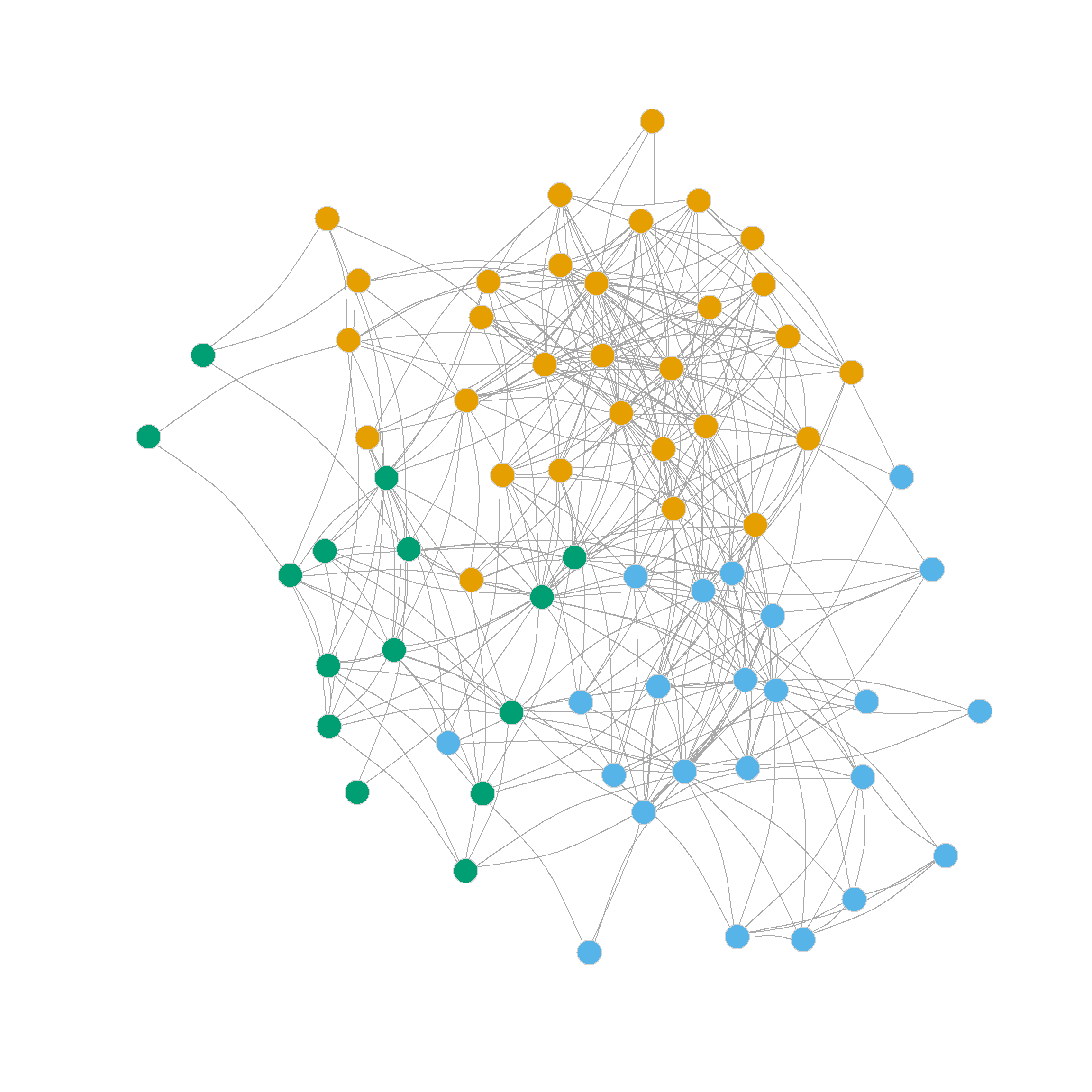
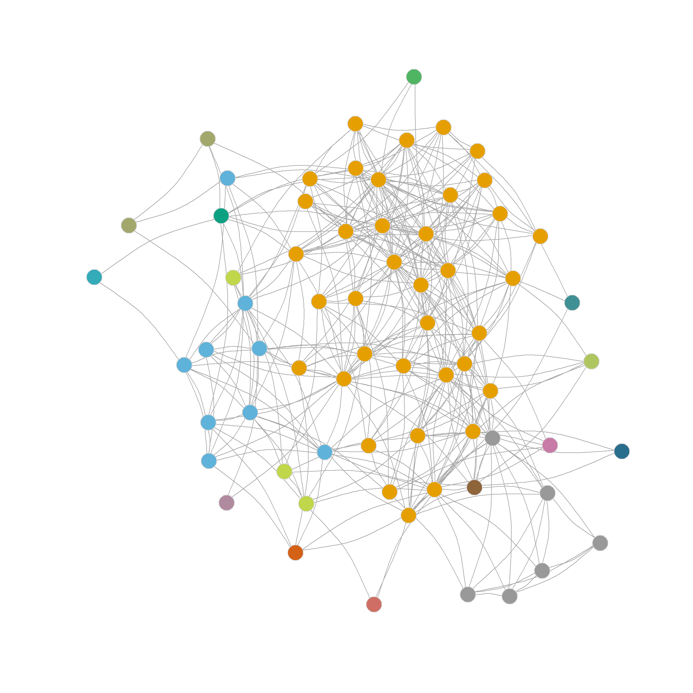
2 2 3 3 3 2 2 3 2 2 2 2 2 2 2 2 Figure 3 shows the results of the three-community partition.
Now let’s say we wanted to check if we should further split any of these three communities into two. All we need to do is create “dummy” variables for the new three community partition and feed these (and the three community membership vector) to the split.mult function, while keeping the original modularity matrix (Newman 2006a):
   c1 <- rep(0, length(s$v))
   c2 <- rep(0, length(s$v))
   c3 <- rep(0, length(s$v))
   c1[which(s$v==1)] <- 1
   c2[which(s$v==2)] <- 1
   c3[which(s$v==3)] <- 1
   dummies <- cbind(c1, c2, c3)
   s <- split.mult(B = Bu,
                   vol = sum(as.matrix(as_adjacency_matrix(ug))),
                   u = dummies,
                   v = s$v)
   s
$delta.Q
[1] 0.000 0.000 -0.002
$v
1 2 3 4 5 6 7 8 9 10 11 12 13 14 15 16 17 18 19 20 21 22 23 24 25 26
1 1 1 1 1 3 3 1 1 1 1 1 1 1 1 1 1 3 1 1 1 1 1 1 1 1
27 28 29 30 31 32 33 34 35 36 37 38 39 40 41 42 43 44 45 46 47 48 49 50 51 52
1 3 1 1 3 3 3 1 3 3 1 2 1 2 2 1 2 2 2 2 3 3 2 2 2 2
53 54 55 56 57 58 59 60 61 62 63 64 65 66 67 68
2 2 3 3 3 2 2 3 2 2 2 2 2 2 2 2
$split
list()Here, the three modularity-split checks failed, as indicated by the delta.Q vector. So no further splits were made (hence the split object is an empty list). This tells us that, according to this method, three communities are the optimal partition.
Of course, if you are working on your project, you don’t have to mess with all of the functions above, because igraph has implemented Newman’s leading eigenvector (of the modularity matrix) community detection method (Newman 2006a) in a single function called cluster_leading_eigen.
To use it, just feed it the relevant graph:
And examine the membership object stored in the results list:
 1  2  3  4  5  6  7  8  9 10 11 12 13 14 15 16 17 18 19 20 21 22 23 24 25 26
 1  1  1  1  1  2  2  1  1  1  1  1  1  1  1  1  1  2  1  1  1  1  1  1  1  1
27 28 29 30 31 32 33 34 35 36 37 38 39 40 41 42 43 44 45 46 47 48 49 50 51 52
 1  2  1  1  2  2  2  1  2  2  1  3  1  3  3  1  3  2  3  3  2  2  3  3  3  3
53 54 55 56 57 58 59 60 61 62 63 64 65 66 67 68
 3  3  2  2  2  3  3  2  3  3  3  3  3  3  3  3
Which returns identical community assignments as above (but with the labels between communities 2 and 3 flipped).
Communities versus Exogenous Attributes
Remember, we began this handout using an exogenous criterion (law firm status as partner or associate) to examine the network’s community structure (which performs pretty well according to modularity). But now we have also used a pure link-based approach to finding communities. How do they compare? Here’s a way to find out:
   library(kableExtra)
   t <- table(V(ug)$status, le.res$membership)
   kbl(t, row.names = TRUE, align = "c", format = "html") %>%
      column_spec(1, bold = TRUE) %>%
      kable_styling(full_width = TRUE,
bootstrap_options = c("hover", "condensed", "responsive"))| 1 | 2 | 3 | |
|---|---|---|---|
| 1 | 27 | 9 | 0 |
| 2 | 3 | 7 | 22 |
This is just a contingency table listing status in the rows (1 = partner) and the three leading eigenvector communities in the columns.
We find that community one (the most coherent, in orange) comprises 89% of partners. So it is a high-status clique. Community three (in blue), on the other hand, is composed entirely of associates, a less dense but completely homogeneous, low-status clique. Finally, community two (green) is a status-mixed clique, composed of nine partners and seven associates.
So in this network, both status and endogenous group dynamics seem to be at play.
An Agglomerative Approach Based on the Modularity
The leading eigenvector approach discussed above is a divisive clustering algorithm. All nodes begin in one community; we split into two, then try to split one of those two into two others (if the modularity increases), and so forth.
But as we noted in the previous handout, another way to cluster is bottom up. All nodes begin in their own singleton cluster, and we join nodes if they maximize some criterion, in this case, the modularity. We then join new nodes to that group. If they increase the modularity, we try other joins, merging communities as we go, until we can’t increase it any further.
This agglomerative approach to clustering is not guaranteed to reach a global maximum, but it can work in most applied settings, even at the risk of getting stuck in a local optimum.
Newman (2004) developed an agglomerative algorithm that optimizes the modularity, a more recent version of which is included in an igraph function called cluster_fast_greedy (Clauset, Newman, and Moore 2004).
Let’s try it out to see how it works:
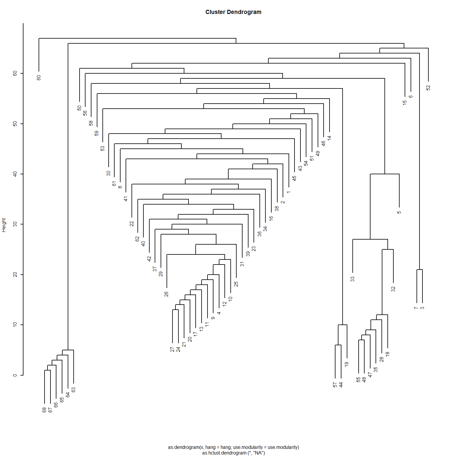
The resulting list object has various sub-objects as components. One of them is called merges, which provides a history of the various merges that led to the final communities. This means we can view the results as a dendrogram, just as we did with structural similarity analyses based on hierarchical clustering of a distance matrix.
To do this, we just transform the resulting object into an hclust object and plot:
This gives us the sense that the network is divided into three communities, as we saw earlier. If we wanted to see which nodes are in which, we could just cut the dendrogram at \(k = 3\):
 1  2  3  4  5  6  7  8  9 10 11 12 13 14 15 16 17 18 19 20 21 22 23 24 25 26
 1  1  2  1  2  2  2  1  1  1  1  1  1  2  1  1  1  2  1  1  1  1  1  1  2  1
27 28 29 30 31 32 33 34 35 36 37 38 39 40 41 42 43 44 45 46 47 48 49 50 51 52
 1  2  1  2  2  2  2  1  2  2  1  3  1  3  3  3  3  3  3  3  2  2  3  1  3  3
53 54 55 56 57 58 59 60 61 62 63 64 65 66 67 68
 3  3  3  2  3  3  3  2  3  3  3  3  3  3  3  3
This provides the relevant assignment to communities (if we wanted more communities, we would cut the tree at a lower height).
Of course, this information was already stored in our results in the membership object:
1 2 3 4 5 6 7 8 9 10 11 12 13 14 15 16 17 18 19 20 21 22 23 24 25 26
1 1 2 1 2 2 2 1 1 1 1 1 1 2 1 1 1 2 1 1 1 1 1 1 2 1
27 28 29 30 31 32 33 34 35 36 37 38 39 40 41 42 43 44 45 46 47 48 49 50 51 52
1 2 1 2 2 2 2 1 2 2 1 3 1 3 3 3 3 3 3 3 2 2 3 1 3 3
53 54 55 56 57 58 59 60 61 62 63 64 65 66 67 68
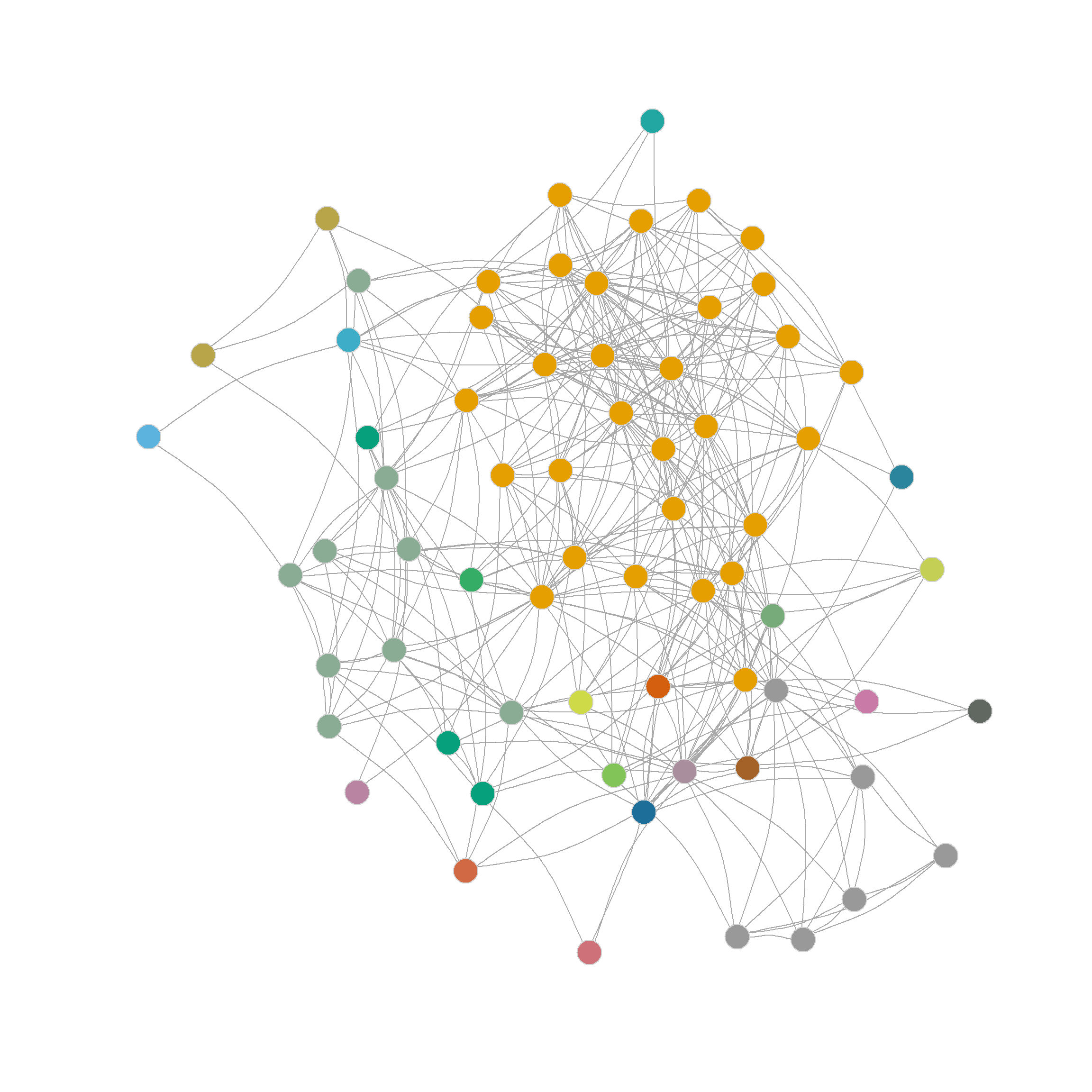
3 3 3 2 3 3 3 2 3 3 3 3 3 3 3 3 Figure 4 visualizes the resulting three-community partition, which is pretty close to what we got using the leading eigenvector method.
Community Detection Using Edge Betweenness
A final approach to community detection with good sociological bona fides relies on edge betweenness, a concept we covered on the lecture notes on betweenness centrality. An edge has high betweenness if many other pairs of nodes need to use it to reach one another via shortest paths.
It follows that if we iteratively identify high betweenness edges, removing the top one, recalculate the edge betweenness on the resulting edge-deleted subgraph, and remove that top one (or flip a coin if two are tied), we have an algorithm for identifying communities as those subgraphs that end up being disconnected after removing the bridges (Girvan and Newman 2002). Note that, like the leading eigenvector method, this approach is divisive with all nodes starting in a single cluster, then that cluster splits into two, and so forth.
For instance, the function below implements a simple version of the Girvan-Newman edge-betweenness community partition algorithm.
The function takes two inputs: some graph h and the number of community partitions desired c. Line two initializes the counter d which keeps track of the number of components in the graph (the number of disconnected clumps). Then we enter a while loop on lines 3-11. In line 4 we compute the edge betweenness of each edge in the graph (using the igraph function edge_betwenness), line 5 checks to see which one is the biggest, and lines 6-7 are designed to keep a random one in case of a tie (hence we need to set the seed for reproducibility). Line 8 deletes the selected edge, line 9 computes the number of components in the graph (using the igraph function components which returns a list of results), and line 10 sets the value of d to the number of components in the new edge-deleted subgraph (stored in the object comp$no). The while loop stops when the number of components comm$no is equal to the function argument c. Line 12 returns a vector of community membership assignments.
And here’s the function in action in the law firm friendship nomination network, requesting a partition into eight groups:
 [1] 1 1 2 1 1 3 2 1 1 1 1 1 1 1 4 1 1 1 1 1 1 1 1 1 1 1 1 1 1 1 1 1 1 1 1 1 1 1
[39] 1 1 1 1 1 1 1 1 1 1 1 5 1 6 1 1 1 1 1 1 1 7 1 1 8 8 8 8 8 8
We can check the modularity of this partition using the igraph function modularity.
The resulting partition is shown in Figure 5 (a)
Note that edge betweenness provides a different picture of the network’s community structure than the eigenvector-based partitioning method. This is not surprising, as it is based on graph-theoretic principles rather than null-model principles such as modularity. The picture here is of two broad communities (in the middle) surrounded by many smaller islands, including some singletons.
In this respect, we can see that the edge-betweenness algorithm begins by selecting the edges, separating pendant nodes and other peripheral nodes into their own communities, which makes sense, since these are the easiest to disconnect (and the edges connecting them to the graph have the highest betweenness). To reach the “middle” or core of the graph, we need to request a partition into more communities. Figure 5 (b) shows the result of using the eb.comms function above to partition the network into sixteen communities. Which looks a bit better, uncovering some actual groups of nodes in the periphery of the network that nominate one another as friends.
Combining Modularity Maximization and Edge-Betweenness
Of course, it is possible to combine the modularity maximization idea with the edge-betweenness partition idea. This is helpful because we usually do not know the actual number of communities in the network; we want the algorithm to tell us. So the trick is to modify the function eb.comms above to compute the modularity of a given partition at each step and record it in a vector. That way, we can pick the biggest number after going through all of the edges.
A function that does that looks like this:
   eb.comms2 <- function(h, s = 123) {
      k <- 1 #initializing counter
      qv <- 0 #initializing modularity vector
      C <- list() #initializing membership vector list
      E <- ecount(h) #number of edges
      og <- h
      while(k < E) { #do until there are no more edges to delete
         eb <- edge_betweenness(h, directed = FALSE) #computing edge betweenness
         e <- which(eb == max(eb)) #grabbing top betweenness edges
         set.seed(s) #setting seed
         if(length(e) > 1) {e <- sample(e, 1)} #grabbing an edge at random in case of tie
         h <- delete_edges(h, e) #deleting top betweenness edge
         comp <- components(h) #computing number of components of edge-deleted graph
         C[[k]] <- comp$membership #creating new community membership vector based on component membership
         qv[k] <- modularity(og, comp$membership, directed = FALSE) #recomputing modularity of original graph
         k <- k + 1 #increasing counter
         }
      maxqpos <- min(which(qv == max(qv))) #picking partition with maximum modularity
      q <- qv[maxqpos] #picking partition with maximum modularity
      membership <- C[[maxqpos]] #picking membership vector with maximum modularity
      nc <- max(membership)
      return(list(q = q, nc = nc, membership = membership))
      }
The main additions here are lines 14 and 15. Line 14 puts the membership vector for the components of the graph in a list object called C at each step (the list is initialized to an empty list in line 4). Line 15 computes the modularity (using the igraph function modularity) on the original graph (not the vertex-deleted one), called og (get it?) initialized in line 6, but using the membership vector from the components of the vertex-deleted subgraph at a given step as community assignments. After the while loop ends (going through all the edges), lines 18-21 grab the community assignments corresponding to the maximum number stored in the modularity vector qv, and line 22 returns the membership vector, a scalar recording the number of communities (the maximum number in the membership vector), and the modularity value as a list object.
Let’s see the new and improved algorithm in action:
$q
[1] 0.2078357

$nc
[1] 23

$membership
 [1]  1  1  2  1  3  4  2  1  1  1  1  1  1  5  6  1  1  3  7  1  1  1  1  1  1
[26]  1  1  3  1  8  1  3  3  1  3  1  1  1  1  1  1  1  9  7 10 11  3  3 12 13
[51] 14 15 16 17  3 18  7 19 20 21 22  1 23 23 23 23 23 23
Which tells us that the optimal partition according to the edge betweenness is one that splits the graph into 23 communities, with a maximum modularity of Q = 0.208.
Of course, all of these steps are packaged in the igraph function called cluster_edge_betweenness. Let’s see how that works.
Note that the cluster_edge_betweenness function takes a graph as input. We have to tell it that is an undirected graph by setting the argument directed to FALSE.
And as we can see, the results are exactly the same we obtained earlier, dividing the nodes in the network into 23 communities. :
 [1]  1  1  2  1  3  4  2  1  1  1  1  1  1  5  6  1  1  3  7  1  1  1  1  1  1
[26]  1  1  3  1  8  1  3  3  1  3  1  1  1  1  1  1  1  9  7 10 11  3  3 12 13
[51] 14 15 16 17  3 18  7 19 20 21 22  1 23 23 23 23 23 23
Interestingly, even though the Girvan-Newman approach is clearly a divisive algorithm, the results can be presented as a dendrogram, but storing top-down divisions rather than bottom-up merges. This is shown in Figure 6
Another thing we can do with the edge_betweenness function output is highlight the edges identified as bridges during the divisive process, since this information is stored in the bridges object. We can use this vector of edge ids to create an edge color vector that will highlight the bridges in red. This is shown in Figure 5 (d).
References
Brandes, Ulrik, Daniel Delling, Marco Gaertler, Robert Gorke, Martin Hoefer, Zoran Nikoloski, and Dorothea Wagner. 2007. “On Modularity Clustering.” IEEE Transactions on Knowledge and Data Engineering 20 (2): 172–88.
Clauset, Aaron, Mark EJ Newman, and Cristopher Moore. 2004. “Finding Community Structure in Very Large Networks.” Physical Review E—Statistical, Nonlinear, and Soft Matter Physics 70 (6): 066111.
Girvan, Michelle, and Mark EJ Newman. 2002. “Community Structure in Social and Biological Networks.” Proceedings of the National Academy of Sciences 99 (12): 7821–26.
Lazega, Emmanuel. 2001. The Collegial Phenomenon: The Social Mechanisms of Cooperation Among Peers in a Corporate Law Partnership. Oxford University Press.
Newman, Mark EJ. 2004. “Fast Algorithm for Detecting Community Structure in Networks.” Physical Review E—Statistical, Nonlinear, and Soft Matter Physics 69 (6): 066133.
———. 2006a. “Finding Community Structure in Networks Using the Eigenvectors of Matrices.” Physical Review E—Statistical, Nonlinear, and Soft Matter Physics 74 (3): 036104.
———. 2006b. “Modularity and Community Structure in Networks.” Proceedings of the National Academy of Sciences 103 (23): 8577–82.
Footnotes
Actually, this is not true; finding the partition that maximizes the modularity in a graph is an NP hard problem (Brandes et al. 2007), so this is just a pretty good approximation of that.↩︎