Using Cliques to Assign Nodes to Overlapping Communities
Palla et al. (2005) provide a simple and intuitive way to partition a network into overlapping communities. The basic idea is to leverage the fact that cliques in a network (fully connected subgraphs of size \(k\)) are likely to share nodes (hence this approach is commonly referred to as the clique percolation method). Communities can then be defined as a clique-concatenation, with linkages between cliques determined by a set of shared members \(q\), typically set to \(k-1\).
Let’s see how this works. First, let’s load up the friendship nomination network from Lazega (2001), constrained to be undirected:
What Palla et al. (2005) propose is to build communities from a set of maximal cliques (fully connected subgraphs of a given size \(k\) that are themselves not subsets of a larger fully connected subgraph).
So the first thing we need to do is settle on a value of \(k\), here we use \(k = 6\).
1 Finding Maximal Cliques and Creating a Bi-Adjacency Matrix
And now we can use the igraph function max_cliques to find all of the maximal cliques of that size:
We can see that there are 24 maximal cliques of size 6 by querying the length of the list returned by the max_cliques function (containing the node ids of the members of each clique as entries). We now have all of the information necessary to create our clique overlap matrix.
The first step is to create a bi-adjacency matrix representing the two-mode network of people and the cliques they belong to (see here). To do that, we first create an empty bi-adjacency matrix full of zeros called B of dimensions 68 by 24, loop through the list of maximal cliques we created earlier called cliques, and insert a one in the corresponding row/column combination:
Code
      [,1] [,2] [,3] [,4] [,5] [,6] [,7] [,8] [,9] [,10]
 [1,]    0    0    0    0    0    0    0    0    0     0
 [2,]    0    0    0    0    0    1    0    0    0     0
 [3,]    0    0    0    0    0    0    0    0    0     0
 [4,]    0    0    0    1    1    1    1    0    0     0
 [5,]    0    0    0    0    0    0    0    0    0     0
 [6,]    0    0    0    0    0    0    0    0    0     0
 [7,]    0    0    0    0    0    0    0    0    0     0
 [8,]    0    0    0    0    0    0    0    0    0     0
 [9,]    0    0    0    0    0    0    0    0    0     0
[10,]    0    0    0    0    0    0    0    0    0     0
The matrix B now has a 1 in the corresponding cell if the row person belongs to the column clique, and 0 otherwise.
We can now use the standard projection approach due to Breiger (1974) to create a clique-by-clique overlap matrix (see here):
      [,1] [,2] [,3] [,4] [,5] [,6] [,7] [,8] [,9] [,10]
 [1,]    6    0    0    0    0    0    0    1    1     1
 [2,]    0    6    0    0    0    0    0    3    3     2
 [3,]    0    0    6    1    0    0    0    1    0     0
 [4,]    0    0    1    6    2    1    2    1    0     0
 [5,]    0    0    0    2    6    4    5    0    0     0
 [6,]    0    0    0    1    4    6    5    0    0     0
 [7,]    0    0    0    2    5    5    6    0    0     0
 [8,]    1    3    1    1    0    0    0    6    5     4
 [9,]    1    3    0    0    0    0    0    5    6     5
[10,]    1    2    0    0    0    0    0    4    5     6
2 Binarizing the Clique Overlap Matrix
Next, we binarize the clique overlap matrix M in three steps. First, we set the diagonal elements of the overlap matrix to zero. Second, we set to zero the entries corresponding to pairs of cliques that have overlap at most \(q = k-1\). Finally, we set to one all the remaining non-zero entries:
Our overlapping communities are the connected components of the resulting binarized clique graph:
Code
 1  2  3  4  5  6  7  8  9 10 11 12 13 14 15 16 17 18 19 20 21 22 23 24
1 2 3 4 5 5 5 6 6 6 7 7 7 8 7 9 10 9 11 12 7 12 12 12 [1] 12We can see that the analysis resulted in 12 overlapping clique communities.
Now, we create a list object containing the node ids for each of the 12 communities, merging together (using the native R function union) the nodes of the overlapping cliques that belong to the same component of the clique overlap graph:
And here are the node IDs of each of the 12 communities:
[[1]]
+ 6/68 vertices, named, from 01e801a:
[1] 68 63 67 66 65 64

[[2]]
+ 6/68 vertices, named, from 01e801a:
[1] 46 40 41 62 53 49

[[3]]
+ 6/68 vertices, named, from 01e801a:
[1] 35 28 31 55 48 32

[[4]]
+ 6/68 vertices, named, from 01e801a:
[1] 23 4  27 24 13 31

[[5]]
+ 8/68 vertices, named, from 01e801a:
[1] 16 12 17 4  21 13 22 2

[[6]]
+ 8/68 vertices, named, from 01e801a:
[1] 51 49 62 31 53 63 61 54

[[7]]
+ 9/68 vertices, named, from 01e801a:
[1] 54 13 24 49 62 40 63 31 26

[[8]]
+ 6/68 vertices, named, from 01e801a:
[1] 2  12 26 24 17 10

[[9]]
+ 7/68 vertices, named, from 01e801a:
[1] 20 17 27 39 11 21 42

[[10]]
+ 6/68 vertices, named, from 01e801a:
[1] 17 27 24 26 13 42

[[11]]
+ 6/68 vertices, named, from 01e801a:
[1] 13 24 27 11 62 4

[[12]]
+ 9/68 vertices, named, from 01e801a:
[1] 13 24 27 26 31 37 29 4  25
3 Creating the Community Membership Bi-Adjacency Matrix
Next, we create a two-mode bi-adjacency matrix Z containing the membership of each node in each of the twelve communities:
The column sums of the Z matrix give us the size of each community:
The row sums of the Z matrix give us the number of communities each node belongs to:
 [1] 0 2 0 4 0 0 0 0 0 1 2 2 6 0 0 1 4 0 0 1 2 1 1 6 1 4 5 1 1 0 5 1 0 0 1 0 1 0
[39] 1 2 1 2 0 0 0 1 0 1 3 0 1 0 2 2 1 0 0 0 0 0 1 4 3 1 1 1 1 1
We can see that some nodes do not belong to any of the communities (they are isolates in the two-mode node-by-community network), so we reduce the Z matrix to get rid of them:
This retains 41 out of the original 68 nodes in the network.
We can now create a subgraph of the original graph containing only those nodes
Finally, we can use some fancy igraph pie chart plotting to visualize the mixed memberships of each node in each community:
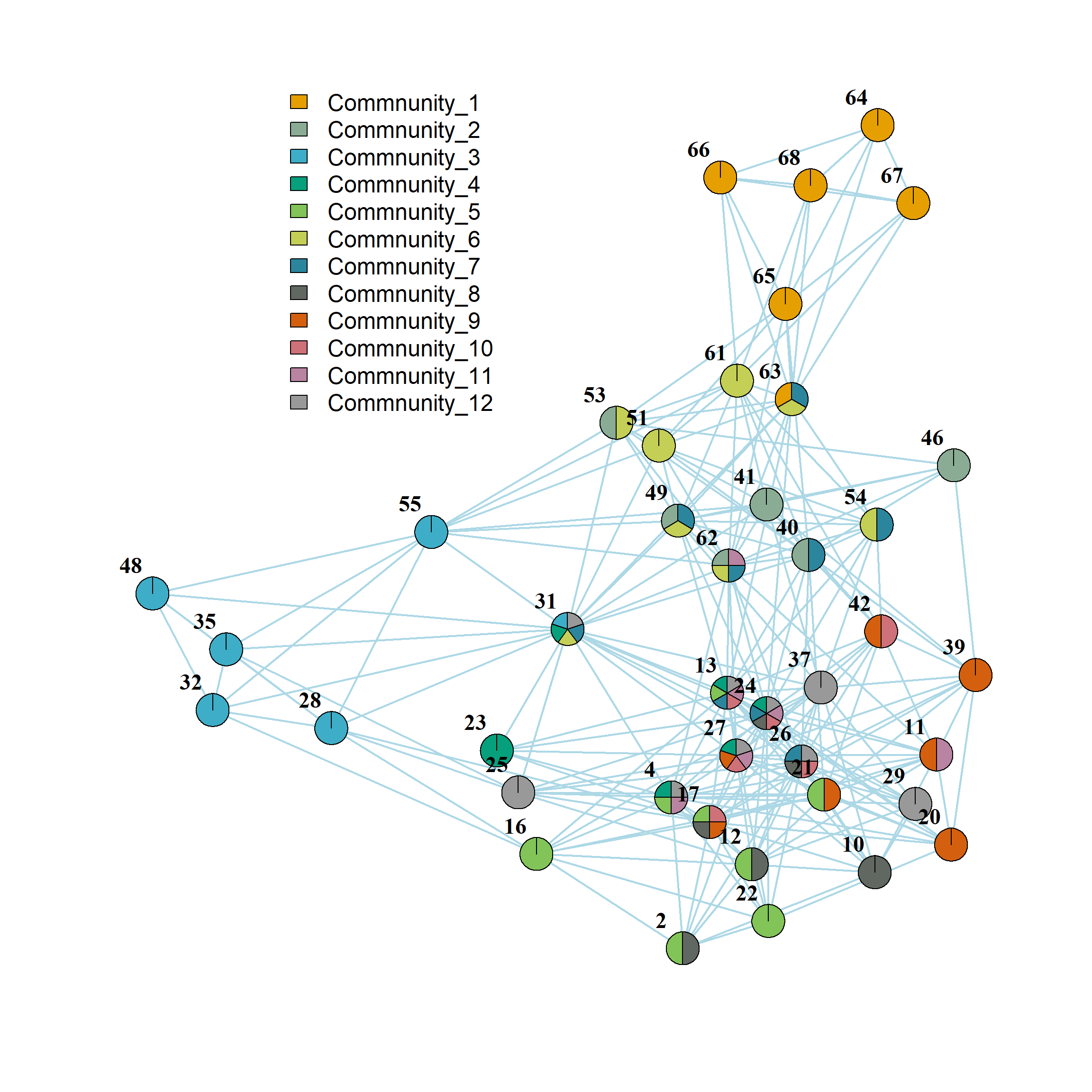
We can see for instance that some sets of nodes (e.g., {64, 65, 66, 67, 68} and {28, 32, 35, 48, 55}) belong to communities with minimal overlap with others (closer to classical communities), while other nodes (e.g., 31 and 13) stand in the middle of multiple communities, centrally located at their intersection.