The Centrality Cube
Brandes et al. (2016) discuss the centrality “cube,” an interesting and intuitive way to understand the way betweenness centrality works, as well as the dual connection between closeness and betweenness.
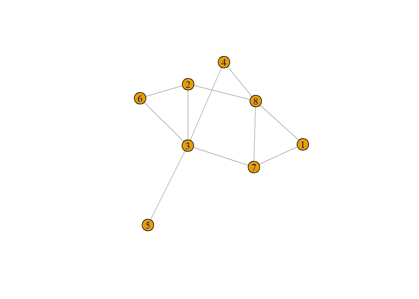
Let us illustrate using a simple example. We begin by creating an Erdos-Renyi graph with eight nodes and connection probability \(p = 0.5\):
The resulting graph looks like:
The basic innovation behind the centrality cube is to store the intermediation information among every node triplet in the graph \(s\), \(r\), \(b\) (standing for “sender,” receiver,” and “broker”) in a three dimensional array rather than the usual two dimensional matrix.
The three dimensional array can be thought of as a “cube” by stacking multiple reachability matrices between every pair of nodes \(s\) and \(r\) along a three dimensional dimension \(b\). So each “b-slice” of the cube will contain the number of times node \(b\) stands in a shortest path between \(s\) and \(r\) divided by the total number of paths between \(s\) and \(r\) which as you recall from our discussion of betweenness centrality computes the pairwise dependence (Brandes 2008) of \(s\) and \(r\) with respect to \(b\).
Let’s see how that works.
1 Building the Cube
We begin by writing a simple user-defined function to compute the number of shortest paths between every pair of nodes in the graph. We need to do this because the cube is built on the ratio of the number of paths that go through a broker node \(b\) to the total number of paths between \(s\) and \(r\):
Code
nsp <- function(w) {
  n <- vcount(w) # number of nodes in the graph
  nodes <- 1:n # vector of node ids
  P <- matrix(1, nrow = n, ncol = n) # initializing the matrix of paths with ones
  for (s in nodes) {
    r <- setdiff(nodes, c(s, as.numeric(neighbors(w, s)))) # non-neighbors in upper triangle
    if (length(r) > 0) {
      P[s, r] <- 0 # Set sr to 0 for disconnected nodes
      vpaths <- all_shortest_paths(w, from = s, to = r)$vpaths
      if (length(vpaths) > 0) {
        dests <- unlist(lapply(vpaths, function(x) as.numeric(x[length(x)])))
        counts <- table(dests)
        P[s, as.numeric(names(counts))] <- as.numeric(counts)
      }
    }
  }
  P[lower.tri(P)] <- t(P)[lower.tri(P)] # copying upper triangle into lower triangle
  return(P)
}
The function is called nsp and takes a graph w as input and returns and matrix called \(\mathbf{P}\) with entries \(p_{sr}\) equal to the total number of shortest paths between \(s\) and \(r\). This is done in four steps:
First, we initialize an \(n \times n\) matrix of ones called \(P\) in line 4 to the all ones matrix. We will update the entries of this matrix with the actual number of shortest paths between each pair of nodes in the graph.
Next, we loop through each node \(s\) in the graph starting in line 5. For each node \(s\), we find the set of target nodes that are not neighbors of \(s\) using the
neighborsfunction inigraphand thesetdifffunction in baseRin line 6. We then check if the set of receiver nodes is not empty using the baseRlengthfunction in line 7, setting the initial value of \(p_{sr}\) to zero for all non-neighboring pairs in line 8.Next, we compute the shortest paths from node \(s\) to the receiver nodes using the
all_shortest_pathsfunction inigraphin line 9. This function returns a list of paths in the objectvpaths, where each path is represented as a vector of node ids. We check if this list is empty or not in line 10. If the list is not empty, we extract the destination nodes from the paths usinglapplyandunlistin line 11, and then count the number of paths to each destination node using the baseRfunctiontablein line 12.Finally, we update the corresponding entries in the \(P\) matrix with the counts of paths in line 13. After going through all nodes, we copy the upper triangle of the \(P\) matrix to the lower triangle to ensure symmetry in line 17, and return the final \(P\) matrix.
Let’s see the function in action:
     [,1] [,2] [,3] [,4] [,5] [,6] [,7] [,8]
[1,]    1    1    1    1    1    2    1    1
[2,]    1    1    1    2    1    1    2    1
[3,]    1    1    1    1    1    1    1    3
[4,]    1    2    1    1    1    1    2    1
[5,]    1    1    1    1    1    1    1    3
[6,]    2    1    1    1    1    1    1    1
[7,]    1    2    1    2    1    1    1    1
[8,]    1    1    3    1    3    1    1    1
Great! Looks like it works.
Now we are ready to write a user defined function to build the cube. Here’s a working example:
Code
cube <- function(w) {
  n <- vcount(w) # number of nodes
  c <- array(0, dim = c(n, n, n)) # initializing the cube with zeros
  S <- nsp(w) # computing number of shortest paths between nodes
  for (s in 1:n) {
    neigh_s <- neighbors(w, s) # pre-fetch neighbors
    for (r in 1:n) {
      if (s != r && !(r %in% neigh_s)) {
        p.sr <- all_shortest_paths(w, s, r)$vpaths
        brokers <- unlist(lapply(p.sr, function(x) as.numeric(x[-c(1, length(x))])))
        if (length(brokers) > 0) {
          b_counts <- table(brokers)
          b_idx <- as.numeric(names(b_counts))
          c[s, r, b_idx] <- as.numeric(b_counts) / S[s, r]
        }
      }
    }
  }
  c[is.na(c)] <- 0
  return(c)
}
The function cube takes a graph w as input and returns a three-dimensional array c with dimensions \(n \times n \times n\) where \(n\) is the number of nodes in the graph. The entries of the array correspond to the pairwise dependence of sender node \(s\) and receiver node \(r\) on broker node \(b\) for all triplets of nodes in the graph.
The function works as follows:
First, we initialize the cube as a three-dimensional array of zeros with dimensions \(n \times n \times n\) in line 3. In line 4, we also compute the matrix \(S\) containing the number of shortest paths between every pair of nodes in the graph using the
nspfunction defined earlier.Next, we loop through each sender node \(s\) in line 5. For each sender node, we pre-fetch its neighbors to speed up the check for non-neighboring receiver nodes in line 6. We then loop through each potential receiver node \(r\) in line 7. We check if \(s\) and \(r\) are different and not neighbors in line 8. If they are valid sender-receiver pairs, we compute all shortest paths from \(s\) to \(r\) using the
all_shortest_pathsfunction in line 9. We then extract the broker nodes from these paths by removing the source and destination nodes usinglapplyandunlistin line 10. If there are any broker nodes, we count how many times each broker node appears in the paths usingtablein line 11, and then update the corresponding entries in the cube with the ratio of the counts to the total number of shortest paths \(S[s, r]\) in line 12.Finally, we replace any
NAvalues in the cube with zeros in line 13 (this can happen if there are no paths between \(s\) and \(r\)), and return the cube in line 14.
2 Exploring the Cube
Once we have our array, we can create all kinds of interesting sub-matrices containing the intermediation information in the graph by summing rows and columns of the array along different dimensions.
First, let us see what’s in the cube. We can query specific two-dimensional sub-matrices using an extension of the usual format for querying matrices in R for three-dimensional arrays. For instance this:
     [,1] [,2] [,3] [,4] [,5] [,6] [,7] [,8]
[1,]  0.0    0 0.00    0 0.00  0.5    0 0.00
[2,]  0.0    0 0.00    0 0.00  0.0    0 0.00
[3,]  0.0    0 0.00    0 0.00  0.0    0 0.33
[4,]  0.0    0 0.00    0 0.00  0.0    0 0.00
[5,]  0.0    0 0.00    0 0.00  0.0    0 0.33
[6,]  0.5    0 0.00    0 0.00  0.0    0 1.00
[7,]  0.0    0 0.00    0 0.00  0.0    0 0.00
[8,]  0.0    0 0.33    0 0.33  1.0    0 0.00
Creates a three-dimensional matrix of pairwise betweenness probabilities and assigns it to the srb object in line 1, and looks at the \(s_{} \times r_{} \times b_2\) entry in line 2.
Each entry in the matrix is the probability that node 2 stands on a shortest path between the row sender and the column receiver node. For instance, the 0.33 in the entry corresponding to row 5 and column 8 tells us that node 2 stands in one third of the shortest paths between nodes 5 and 8 (there are 3 distinct shortest paths between 5 and 8).
Because each sub-matrix in the cube is a matrix, we can do the usual matrix operations on them. For instance, let’s take the row sums of the \(s\) to \(r\) matrix corresponding to node 3 as the broker. This can be done like this:
  1   2   3   4   5   6   7   8
1.5 2.0 0.0 3.0 6.0 3.5 3.0 1.0
As Brandes et al. (2016), note this vector gives us the one-sided dependence of each node in the graph on node 3. Obviously node 3 doesn’t depend on itself so there is a zero on the third spot in the vector. As is clear from the plot, node 5 is the most dependent on 3 for intermediation with the rest of the nodes in the graph.
We can also pick a particular sender and receiver node and sum all their dyadic entries in the cube across the third (broker) dimension:
This number is equivalent to the geodesic distance between the nodes minus one:
3 Betweenness and Closeness in the Cube
The betweenness centrality of each node is encoded in the cube, because we already computed the main ratio that the measure depends on, namely, the pairwise dependence of each pair of nodes in the graph on any given node. For instance, let’s look at the matrix obtained from taking the slice of cube that corresponds to node 3 as a broker:
     [,1] [,2] [,3] [,4] [,5] [,6] [,7] [,8]
[1,]  0.0  0.0    0  0.0    1  0.5  0.0    0
[2,]  0.0  0.0    0  0.5    1  0.0  0.5    0
[3,]  0.0  0.0    0  0.0    0  0.0  0.0    0
[4,]  0.0  0.5    0  0.0    1  1.0  0.5    0
[5,]  1.0  1.0    0  1.0    0  1.0  1.0    1
[6,]  0.5  0.0    0  1.0    1  0.0  1.0    0
[7,]  0.0  0.5    0  0.5    1  1.0  0.0    0
[8,]  0.0  0.0    0  0.0    1  0.0  0.0    0
The sum of the all the cells in this matrix (divided by two) correspond to node 3’s betweenness centrality:
So to get each node’s betweenness we just can just sum up the entries in each of the cube’s sub-matrices:
Code
    1     2     3     4     5     6     7     8
0.00 2.17 10.00 0.67 0.00 0.00 3.17 4.00 1 2 3 4 5 6 7 8
0.00 2.17 10.00 0.67 0.00 0.00 3.17 4.00 Note the neat trick of using the argument dims = 2 in the usual colSums command. This tells colSums that we are dealing with a three dimensional matrix, and that what we want is the sum of the columns across the cube’s third dimension (the brokers). Note also that we divide the cube betweenness by two because we are summing identical entries across the upper and lower triangle of the symmetric dyadic brokerage matrices inside the cube (not surprisingly, node 3 is the top betweenness centrality node).
As Brandes et al. (2016) point out, using the cube info, we can build a matrix of one-sided dependencies between each pair of nodes. In this matrix, the rows correspond to a sender (or receiver) node, the columns to a broker node and the \(sb^{th}\) entry contains the sum of the proportion of paths containing the broker nodes that starts with the sender node and end with some other node in the graph.
Here’s a function that uses the cube info to build the dependency matrix that Brandes et al. (2016) talk about using the cube as input:
This function just takes the various vectors formed by the row sums of the sender-receiver matrix across each value of the third dimension (which is just each node in the graph when playing the broker role). It then returns a regular old \(n \times n\) containing the info.
Here’s the result when applied to our little example:
Code
| 1 | 2 | 3 | 4 | 5 | 6 | 7 | 8 | |
|---|---|---|---|---|---|---|---|---|
| 1 | 0 | 0.50 | 1.5 | 0.00 | 0 | 0 | 2.50 | 2.5 |
| 2 | 0 | 0.00 | 2.0 | 0.00 | 0 | 0 | 0.00 | 2.0 |
| 3 | 0 | 0.33 | 0.0 | 0.33 | 0 | 0 | 1.33 | 0.0 |
| 4 | 0 | 0.00 | 3.0 | 0.00 | 0 | 0 | 0.00 | 2.0 |
| 5 | 0 | 0.33 | 6.0 | 0.33 | 0 | 0 | 1.33 | 0.0 |
| 6 | 0 | 1.50 | 3.5 | 0.00 | 0 | 0 | 0.50 | 0.5 |
| 7 | 0 | 0.00 | 3.0 | 0.00 | 0 | 0 | 0.00 | 1.0 |
| 8 | 0 | 1.67 | 1.0 | 0.67 | 0 | 0 | 0.67 | 0.0 |
Note that this valued matrix of one-sided dependencies is asymmetric, because the one-dependence of \(i\) on \(j\) does not have to be the same as the one-sided dependency of \(j\) on \(i\). Take for instance, node 3. Every node in the graph depends on node 3 for access to other nodes, but node 3 does not depend on nodes 1, 5, 6, or 8.
Interestingly, as Brandes et al. (2016) also show, the betweenness centrality also can be calculated from the dependency matrix! All we need to do is compute the column sums, equivalent to in-degree in the directed dependence network:
Even more interestingly, closeness centrality is also in the dependence matrix! It is given by the outdegree of each actor in the directed dependence network, corresponding to the row sums of the matrix (shifted by a constant given by \(n-1\)).
Code
    1     2     3     4     5     6     7     8
0.071 0.091 0.111 0.083 0.067 0.077 0.091 0.091 1 2 3 4 5 6 7 8
0.071 0.091 0.111 0.083 0.067 0.077 0.091 0.091 Here we see that node 3 is also the top in closeness, followed closely (pun intended) by nodes 2, 7, and 8. This makes sense because an actor with high closeness is one that has low dependence on key nodes to be able to reach others.
Of course, closeness is also in the cube because of the mathematical relationship we saw earlier between the sum of entries between senders and receivers across brokers in the cube and the geodesic distance.
For instance, let’s get the matrix corresponding to node 3’s role as sender across all brokers and receivers:
     [,1] [,2] [,3] [,4] [,5] [,6] [,7] [,8]
[1,]    0 0.00    0 0.00    0    0 1.00    0
[2,]    0 0.00    0 0.00    0    0 0.00    0
[3,]    0 0.00    0 0.00    0    0 0.00    0
[4,]    0 0.00    0 0.00    0    0 0.00    0
[5,]    0 0.00    0 0.00    0    0 0.00    0
[6,]    0 0.00    0 0.00    0    0 0.00    0
[7,]    0 0.00    0 0.00    0    0 0.00    0
[8,]    0 0.33    0 0.33    0    0 0.33    0
The entries of this matrix give us the probability that node 3 is the sender, whenever the row node is the is the broker (an inner node in the path) and the column node is the receiver.
For instance, the value 0.3 in row 8 and column 1 tells us that node 3 is the sender node in one third of the paths that end in node 1 and feature node 8 as a broker.
Interestingly, the sums of the entries in this matrix are equivalent to the sum of the geodesic distances between node 3 and every other node in the graph shifted by a constant (\(n- 1\)):
So the closeness centrality can be computed from the cube as follows:
[1] 0.071 0.091 0.111 0.083 0.067 0.077 0.091 0.091Which is the same as: