---
title: "Finding Communities via Edge-Deletion"
---
## Community Detection Using the Edge-Betweenness
Another approach to community detection with good sociological bona fides relies on **edge betweenness**, a concept we covered on the [lecture notes on edge centralities](cent-edge.qmd). An edge has high betweenness if many other pairs of nodes need to use it to reach one another via shortest paths.
It follows that if we iteratively identify high betweenness edges, removing the top one, recalculate the edge betweenness on the resulting edge-deleted subgraph, and remove *that* top one (or flip a coin if two are tied), we have an algorithm for identifying communities as those subgraphs that end up being disconnected after removing the bridges [@girvan_newman02]. Note that, like the leading eigenvector method, this approach is **divisive** with all nodes starting in a single cluster, then that cluster splits into two, and so forth.
For instance, the function below implements a simple version of the Girvan-Newman edge-betweenness community partition algorithm.
```{r}
eb.comms <- function(h, c, s = 123) {
  d <- components(h)$no # computing graph components
  set.seed(s)
  while (d < c) {
    eb <- edge_betweenness(h, directed = FALSE) # computing edge-betweenness vector
    e <- which(eb == max(eb)) # picking largest value
    if (length(e) > 1) {
      e <- sample(e, 1)
    } # grabbing an edge at random in case of tie
    h <- delete_edges(h, e) # deleting to betweenness edge
    comps <- components(h) # computing graph components
    d <- comps$no # number of components
  }
  return(comps$membership) # returning membership vector
}
```
The function takes two inputs: a graph `h` and the desired number of community partitions, `c`. Line two initializes the counter `d` which keeps track of the number of **components** in the graph (the number of disconnected clumps). Then we enter a `while` loop on lines 3-11. In line 4, we compute the **edge betweenness** of each edge in the graph (using the `igraph` function `edge_betweenness`), line 5 checks to see which one is the biggest, and lines 6-7 are designed to keep a random one in case of a tie (hence we need to set the seed for reproducibility). Line 8 deletes the selected edge, line 9 computes the number of components in the graph (using the `igraph` function `components` which returns a `list` of results), and line 10 sets the value of `d` to the number of components in the new **edge-deleted subgraph** (stored in the object `comp$no`). The `while` loop stops when the number of components `comm$no` is equal to the function argument `c`. Line 12 returns a vector of community membership assignments.
And here's the function in action in the law firm friendship nomination network, requesting a partition into eight groups:
```{r}
library(networkdata)
library(igraph)
g <- law_friends
g <- subgraph(g, degree(g) >= 2)
ug <- as_undirected(g, mode = "collapse")
c8 <- eb.comms(ug, c = 8)
c8
```
We can check the modularity of this partition using the `igraph` function `modularity.`
```{r}
modularity(ug, c8)
```
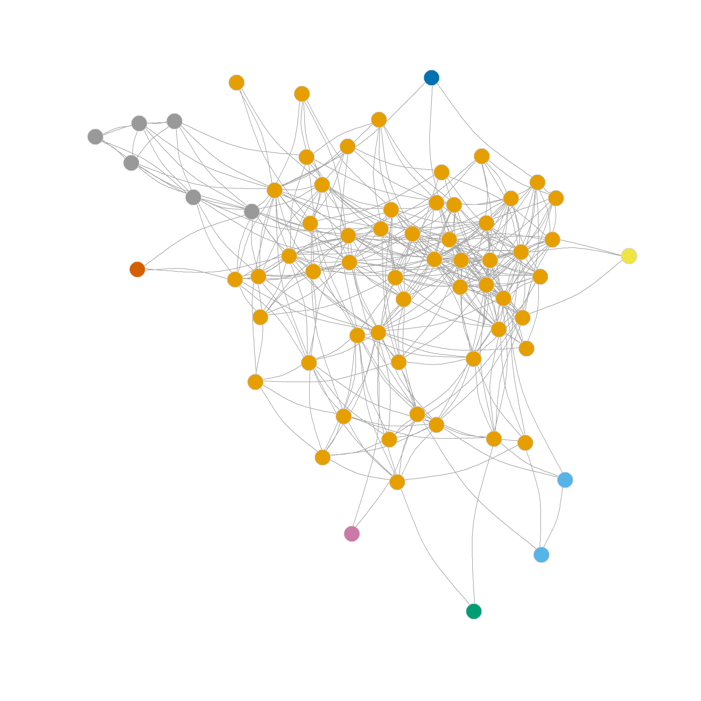
The resulting partition is shown in
Note that edge betweenness provides a different picture of the network's community structure than the eigenvector-based partitioning method. This is not surprising, as it is based on graph-theoretic principles rather than null-model principles such as modularity. The picture here is of two broad communities (in the middle) surrounded by many smaller islands, including some singletons.
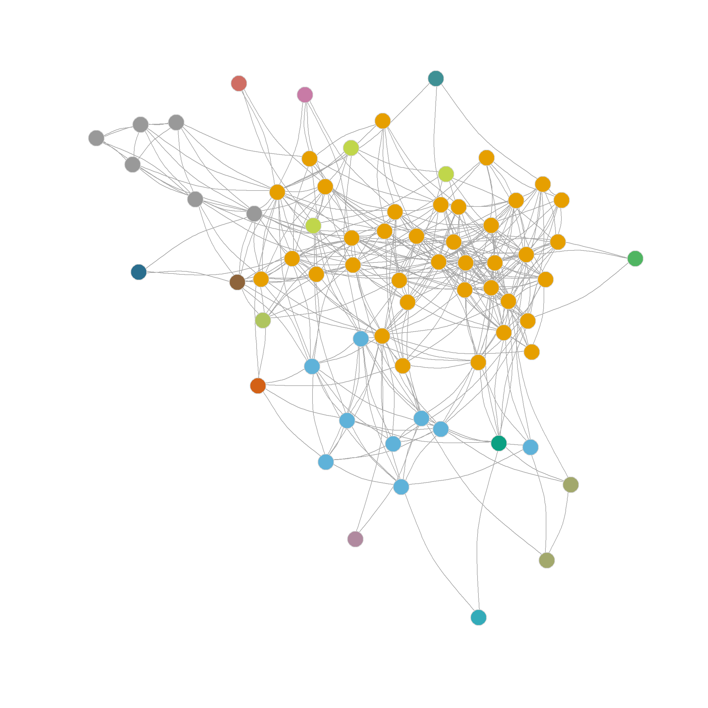
In this respect, we can see that the edge-betweenness algorithm begins by selecting the edges, separating pendant nodes and other peripheral nodes into their own communities, which makes sense, since these are the easiest to disconnect (and the edges connecting them to the graph have the highest betweenness). To reach the "middle" or core of the graph, we need to request a partition into more communities. shows the result of using the `eb.comms` function above to partition the network into sixteen communities. Which looks a bit better, uncovering some actual groups of nodes in the periphery of the network that nominate one another as friends.
## Combining Modularity Optimization and Edge-Betweenness
Of course, it is possible to combine the modularity optimization idea with the edge-betweenness partition idea. This is helpful because we usually do not know the actual number of communities in the network; we want the algorithm to tell us. So the trick is to modify the function `eb.comms` above to compute the modularity of a given partition at each step and record it in a vector. That way, we can pick the biggest number after going through all of the edges.
A function that does that looks like this:
```{r}
eb.comms2 <- function(h, s = 123) {
  k <- 1 # initializing counter
  qv <- 0 # initializing modularity vector
  C <- list() # initializing membership vector list
  og <- h # original graph before deleting edges
  set.seed(s) # setting seed
  while (ecount(h) > 0) { # do until there are no more edges to delete
    eb <- edge_betweenness(h, directed = FALSE) # computing edge betweenness
    top.e <- which(eb == max(eb)) # grabbing top betweenness edges
    if (length(top.e) > 1) {
      top.e <- sample(top.e, 1)
    } # grabbing an edge at random in case of multi-way tie
    h <- delete_edges(h, top.e) # deleting top betweenness edge
    comp <- components(h) # computing number of components of edge-deleted graph
    C[[k]] <- comp$membership # creating new community membership vector based on component membership
    qv[k] <- modularity(og, comp$membership, directed = FALSE) # recomputing modularity of original graph
    k <- k + 1 # increasing counter
  }
  maxqpos <- min(which(qv == max(qv))) # picking partition with maximum modularity
  q <- qv[maxqpos] # picking partition with maximum modularity
  membership <- C[[maxqpos]] # picking membership vector with maximum modularity
  nc <- max(membership)
  return(list(q = q, nc = nc, membership = membership))
}
```
The main additions here are lines 13 and 14. Line 13 puts the membership vector for the graph's components into a list object called `C` at each step (the list is initialized to an empty list in line 4). Line 14 computes the modularity (using the `igraph` function `modularity`) *on the original graph* (not the vertex-deleted one), called `og` (get it?), initialized in line 5, but using the membership vector from the components of the vertex-deleted subgraph at a given step as community assignments. After the `while` loop ends (going through all the edges), lines 17-20 grab the community assignments corresponding to the maximum number stored in the modularity vector `qv`, and line 21 returns a list containing membership vector stored in the object `membership`, a scalar recording the number of communities (the maximum number in the membership vector) stored in the object `nc`, and a scalar recording the maximum modularity value stored in the object `q`.
Let's see the new and improved algorithm in action:
```{r}
c.mod <- eb.comms2(ug)
c.mod
```
Which tells us that the optimal partition according to the edge betweenness is one that splits the graph into `r c.mod$nc` communities, with a maximum modularity of Q = `r round(c.mod$q, 3)`.
Of course, all of these steps are packaged in the `igraph` function called `cluster_edge_betweenness`. Let's see how that works.
```{r}
eb.res <- cluster_edge_betweenness(ug, directed = FALSE)
```
Note that the `cluster_edge_betweenness` function takes a graph as input. We have to tell it that it is an undirected graph by setting the argument `directed` to `FALSE`.
And as we can see, the results are exactly the same we obtained earlier, dividing the nodes in the network into `r max(eb.res$membership)` communities.
:
```{r}
eb.res$membership
```
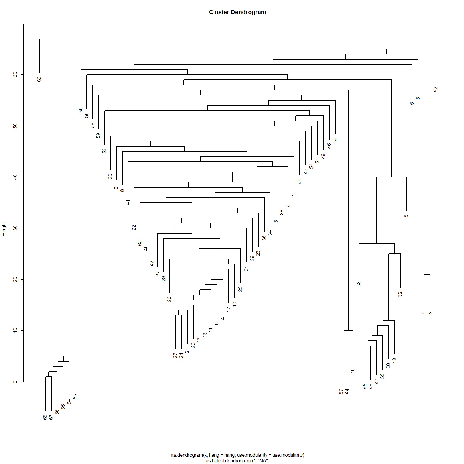
Interestingly, even though the Girvan-Newman approach is clearly a divisive algorithm, the results can be presented as a dendrogram that stores top-down divisions rather than bottom-up merges. This is shown in
```{r}
#| label: fig-ebdendro
#| fig-cap: "Dendrogram of Community Partition of the Law Friends Network Using the Edge-Betweenness."
#| fig-height: 8
#| fig-width: 8
hc <- as.hclust(eb.res)
par(cex = 0.5) # smaller labels
plot(hc)
```
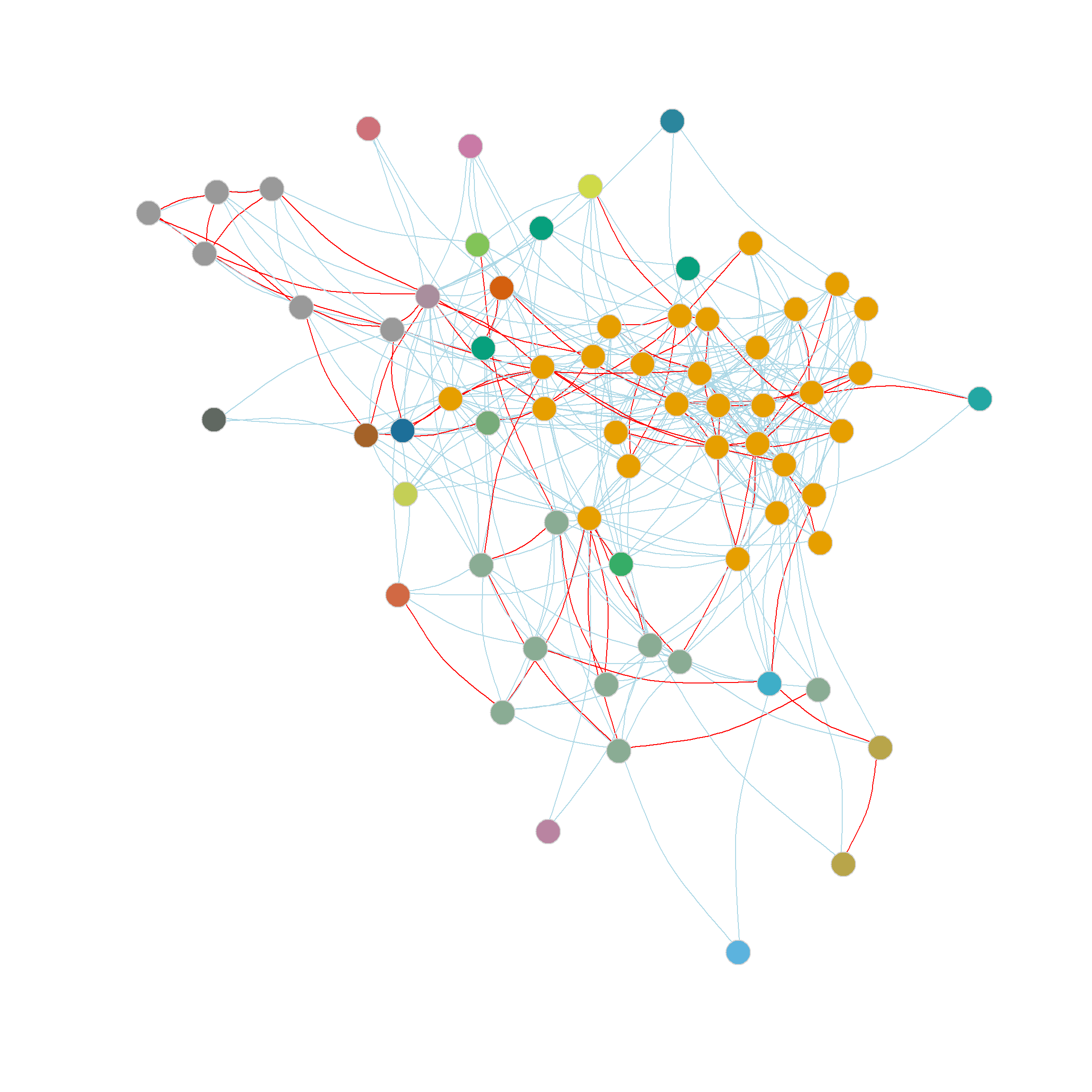
Another thing we can do with the `edge_betweenness` function output is highlight the edges identified as **bridges** during the divisive process, since this information is stored in the `bridges` object. We can use this vector of edge IDs to create an edge-color vector that highlights the bridges in red. This is shown in .
## Community Detection Using the Edge Clustering Coefficient
@radicchi_etal04 propose another version of an edge-deletion approach to community detection based on an edge-level metric they call the **edge clustering coefficient** $C(e_{ij})$. This is essentially a measure of the extent to which an edge connects nodes that themselves share a lot of neighbors, normalized by the minimum of the degrees of the nodes minus one:
$$
C(e_{ij}) = \frac{z_{ij} + 1}{min\left[(k_i - 1), (k_j - 1)\right]}
$$ {#eq-eclust}
Where $z_{ij}$ is the number of common neighbors shared by nodes $i$ and $j$ incident to edge $e_{ij}$, and $k_i$ and $k_j$ are their respective degrees. @radicchi_etal04 add one to the numerator of to account for the fact that some connected nodes may not share any neighbors.
The logic of the @radicchi_etal04 approach is that edges between well-clustered communities should have a *low* edge clustering coefficient (e.g., connecting nodes that themselves don't share many neighbors and therefore belong to different communities). Meanwhile, edges with a high clustering coefficient should be more likely to link nodes that belong to the same community.
Ergo, deleting the edges with low edge clustering coefficient (like we did with the ones that had high edge betweenness) should partition a graph into well-defined communities.
To implement this approach, we need (1) a function to compute the clustering coefficient for each edge according to , and (2) a modification of the `eb.comms2` function above that incorporates the idea of removing edges with minimum edge clustering scores.
To complete step 1, here's a function to compute the edge clustering coefficient as defined by @radicchi_etal04:
```{r}
edge.clust <- function(h) {
  d <- degree(h) # degree vector
  edgemat <- ends(h, E(h)) # edge list matrix
  w <- as.matrix(as_adjacency_matrix(h)) # graph adjacency matrix
  m <- w %*% w # commons neighbors matrix
  ec <- apply(edgemat, 1, function(row) { # applies function to each row of matrix edgemat
    i <- row[1] # first node
    j <- row[2] # second node
    z <- m[i, j] # common neighbors
    return((z + 1) / min((d[i] - 1), (d[j] - 1))) # edge clustering coefficient
  })
  return(ec)
}
```
This function takes some graph `h` as input and returns a vector of length $|E|$ (number of edges in the graph) containing the estimated clustering coefficient of each edge as components. Note that we compute the number of shared neighbors by taking the second power of the adjacency matrix in lines 4 and 5. The `apply` call then iterates over each row of the edgelist (with the second argument set to `1`) and applies the custom edge clustering coefficient function in the third argument.
And to complete step 2, here's a modification of our edge-deletion function above to incorporate the edge clustering coefficient as the criterion for edge deletion:
```{r}
ec.comms <- function(h) {
  qv <- 0 # initializing modularity vector
  C <- list() # initializing membership vector list
  og <- h # original graph before deleting edges
  k <- 1 # initializing counter
  while (ecount(h) > 0) { # do until there are no more edges to delete
    ec <- edge.clust(h) # computing edge clustering coefficient vector
    min.e <- which(ec == min(ec)) # grabbing minimum clustering edges
    h <- delete_edges(h, min.e) # deleting minimum clustering edges
    comp.vec <- components(h)$membership # component membership vector of edge-deleted graph
    C[[k]] <- comp.vec # storing membership vector on list
    qv[k] <- modularity(og, comp.vec, directed = FALSE) # recomputing modularity of original graph using membership vector
    k <- k + 1 # increasing counter
  }
  maxqpos <- min(which(qv == max(qv))) # picking partition with maximum modularity
  q <- qv[maxqpos] # picking partition with maximum modularity
  membership <- C[[maxqpos]] # picking membership vector with maximum modularity
  nc <- max(membership)
  return(list(q = q, nc = nc, membership = membership))
}
```
Note that the main difference between this function and the one we used for the edge betweenness is that instead of flipping a coin and selecting a random edge in case of a tie, we now deterministically kill *all* edges that have minimum clustering (usually zero or a number close to zero) in line 9.
And here are the results for the `law_friends` network:
```{r}
ec <- ec.comms(ug)
ec
```
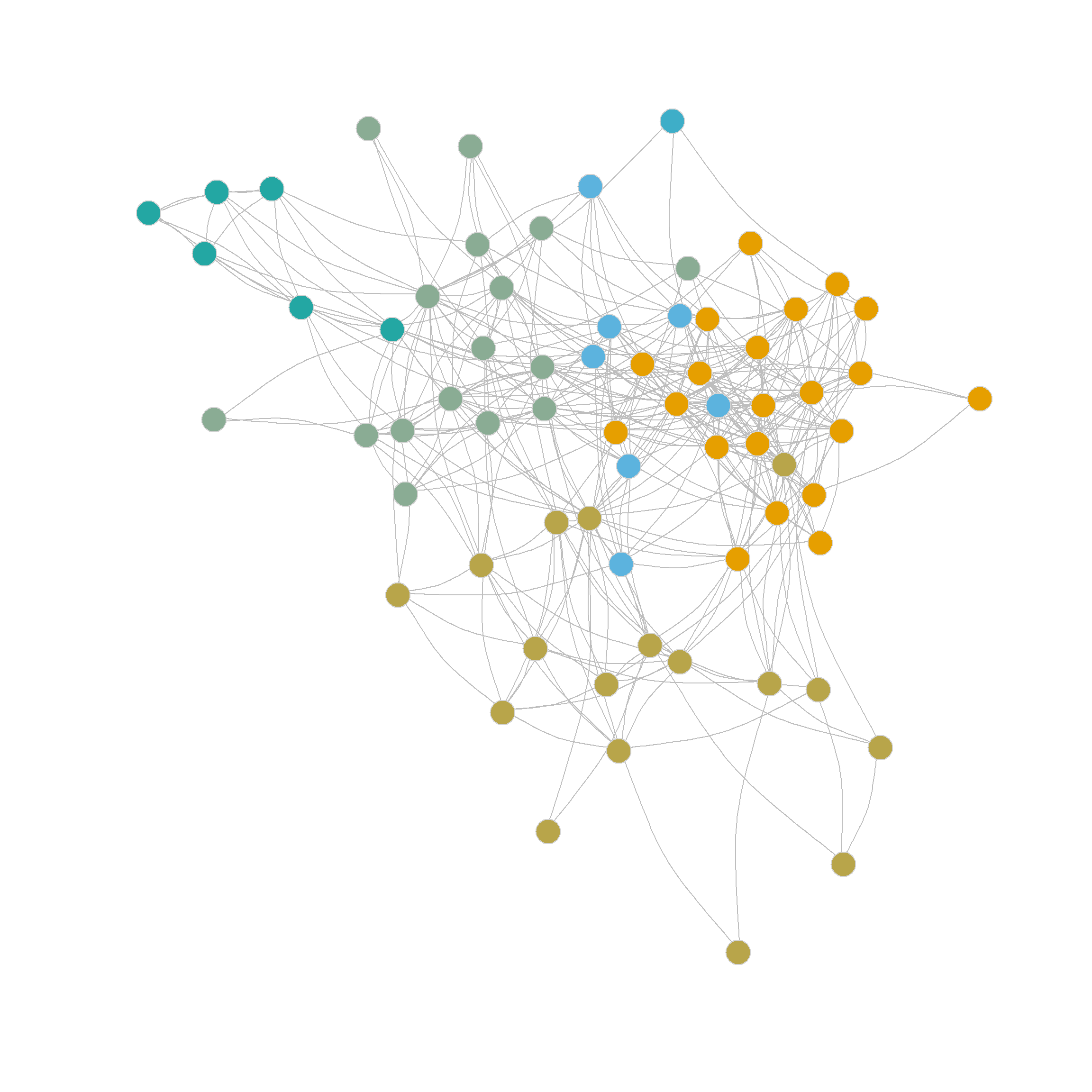
```{r}
#| label: fig-eb
#| fig-cap: "Undirected Law Firm Friendship Network."
#| fig-height: 12
#| fig-width: 12
#| fig-subcap:
#| - "Community Partition According to the Edge Betweenness (C = 8)."
#| - "Community Partition According to the Edge Betweenness (C = 16)."
#| - "Community Partition According to the Edge Betweenness with Maximum Modularity (C = 23)."
#| - "Community Partition According to the Edge Clustering with Maximum Modularity (C = 6)."
#| layout-ncol: 2
#| echo: false
library(RColorBrewer)
set.seed(234)
ul <- layout_with_fr(ug)
V(ug)$color <- c8
plot(ug,
layout = ul,
vertex.size = 6, vertex.frame.color = "lightgray",
vertex.label = NA, edge.arrow.size = 0.25,
vertex.label.dist = 1, edge.curved = 0.2
)
getPalette <- colorRampPalette(categorical_pal(8))
c16 <- eb.comms(ug, c = 16)
pal <- getPalette(max(c16))
V(ug)$color <- c16
ug$palette <- pal
plot(ug,
layout = ul,
vertex.size = 6, vertex.frame.color = "lightgray",
vertex.label = NA, edge.arrow.size = 0.25,
vertex.label.dist = 1, edge.curved = 0.2
)
getPalette <- colorRampPalette(categorical_pal(8))
pal <- getPalette(max(c.mod$membership))
V(ug)$color <- c.mod$membership
ug$palette <- pal
e.col <- rep("lightblue", ecount(ug))
e.col[eb.res$bridges] <- "red"
E(ug)$color <- e.col
plot(ug,
layout = ul,
vertex.size = 6, vertex.frame.color = "lightgray",
vertex.label = NA, edge.arrow.size = 0.25,
vertex.label.dist = 1, edge.curved = 0.2
)
V(ug)$color <- ec$membership
E(ug)$color <- "gray"
plot(ug,
layout = ul,
vertex.size = 6, vertex.frame.color = "lightgray",
vertex.label = NA, edge.arrow.size = 0.25,
vertex.label.dist = 1, edge.curved = 0.2
)
```
Which suggests a partition into `r ec$nc` communities with a modularity score of `r round(ec$q, 3)` outperforming the best edge-betweenness partition by this metric.
shows the resulting communities obtained from the edge-clustering coefficient approach. As shown in the Figure, the edge-clustering coefficient approach produces strongly defined, intuitive communities, grouping together densely connected groups of nodes.